Maximum Likelihood Estimation (MLE)

Introduction

This site provides a brief introduction to maximum likelihood estimation: the details are not essential to learn, but it is useful to have a grasp of some of the underlying principles.

Probability

The concept of likelihood, introduced by Sir R. A. Fisher, is closely related to the more common concept of probability. We speak about the probability of observing events. For example, for an unbiased coin, the probability of observing heads is 0.5 for every toss. This is taken to mean that if a coin were tossed a large number of times then we would expect, on average, to find half of the time the coin landed heads, half of the time tails.

There are certain laws of probability that allow us to make inferences and predictions based on probabilistic information. For example, the probabilities of different outcomes for a certain event must always add up to 1: if there is a 20% chance of rain today, there must be an 80% chance of no rain. Another very common law is that if two events are independent of one another (that is, they in no way influence each other), then the probability of certain pairs of outcomes will be the product of the two outcomes by themselves: if we toss a coin twice, the probability of getting 2 heads is 0.5 times 0.5 = 0.25.

Models: parameters and distributions

When we speak about the probability of observing events such as the outcome of a toss of a coin, we are implicitly assuming some kind of model, even in this simple case. In the case of a coin, the model would state that there is some certain, fixed probability for the particular outcomes. This model would have one parameter, p the probability of the coin landing on heads. If the coin is fair, then p=0.5. We can then speak about the probability of observing an event, given specific parameter values for the model. In this simple case, if p =0.5, then the probability of the coin landing heads on any one toss is also 0.5.

In the case of this simple example, it does not seem that we have gained very much - we seem to be merely calling what was previously a simple probability the parameter of a model. As we shall see, however, this way of thinking provides a very useful framework for expressing more complex problems.

Conditional probability

In the real world, very few things have absolute, fixed probabilities. Many of the aspects of the world that we are familiar with are not truly random. Take for instance, the probability of developing schizophrenia. Say that the prevalence of schizophrenia in a population is 1%. If we know nothing else about an individual, we would say that the probability of this individual developing schizophrenia is 0.01. In mathematical notation,

                   P(Sz) = 0.01

We know from empirical research, however, that certain people are more likely to develop schizophrenia than others. For example, having a schizophrenic first-degree relative greatly increases the risk of becoming schizophrenic. The probability above is essentially an average probability, taken across all individuals both with and without schizophrenic first-degree relatives.

The notion of conditional probability allows us to incorporate other potentially important variables, such as the presence of familial schizophrenia, into statements about the probability of an individual developing schizophrenia. Mathematically, we write


                   P( X | Y)

meaning the probability of X conditional on Y or given Y. In our example, we could write


    P (Sz | first degree relative has Sz)

and


    P (Sz | first degree relative does not have Sz)

Whether or not these two values differ is an indication of the influence of familial schizophrenia upon an individual's chances of developing schizophrenia.

---

Previously, we mentioned that all probability statements depend on some kind of model in some way. The probability of an outcome will be conditional upon the parameter values of this model. In the case of the coin toss,


     P (H | p=0.5)

where H is the event of obtaining a head and p is the model parameter, set at 0.5.

Let's think a little more carefully about what the full model would be for tossing a coin, if p is the parameter. What do we know about coin tossing?

The outcome is a discrete, binary outcome for each toss - it is either heads or tails.
We assume that the probability of either outcome does not change over time.
We assume that the outcome of each toss of a coin can be regarded as independent from all other outcomes. That is, getting five heads in a row does not make it any more likely to get a tail on the next trial.
In the case of a 'fair' coin, we assume a 50:50 chance getting either heads or tails - that is, p=0.5.

Say we toss a coin a number of times and record the number of times it lands on heads. The probability distribution that describes just this kind of scenario is called the binomial probability distribution. It is written as follows :

Let's take a moment to work through this. The notation is as follows:-

n = total number of coin tosses
h = number of heads obtained
p = probability of obtaining a head on any one toss

(The ! symbol means factorial (5! = 1x2x3x4x5 = 120).)

We can think of this equation in two parts. The second part involves the joint probability of obtaining h heads (and therefore n-h tails) if a coin is tossed n times and has probability p of landing heads on any one toss (and therefore probability 1-p of landing tails). Because we have assumed that each of the n trails is independent and with constant probability the joint probability of obtaining h heads and n-h tails is simply the product of all the individual probabilities. Imagine we obtained 4 heads and 5 tails in 9 coin tosses. Then

is simply convenient notation for

The first half of the binomial distribution function is concerned with the fact that there is more than 1 way to get, say, 4 heads and 5 tails if a coin is tossed 9 times. We might observe


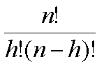
   H, T, H, H, T, T, H, T, T.

 

   T, H, H, T, H, T, T, H, T.

or even

 

   H, H, H, H, T, T, T, T, T.

Every one of the permutations is assumed to have equal probability of occurring - the coefficient

represents the total number of permutations that would give 4 heads and 5 tails.

So, the probability of obtaining 4 heads and 5 tails for a fair coin is

Return to front page
Site created by S.Purcell, last updated 1.10.2000