Behavioural Genetic Interactive Modules
Correlation & Regression

Overview
This module aims to introduce the related concepts of
correlation and regression and to demonstrate their
relationship with variance and covariance.
Tutorial
As mentioned in the previous module, in order to assess the
magnitude of a covariance statistic we can use information
about the variances of the measures to standardise
it. We can also calculate so-called regression
coefficients easily from the covariance if we know the
variance of the measures.
This module allows the user to explore these related
measures by simulating a bivariate dataset with
certain known properties.
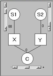
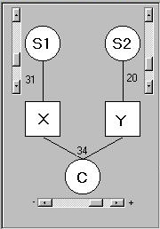 This panel is used to specify the relationship
between the two simulated variables, X and Y. It
represents three separate influences, or sources of
variation, on the two measures:
This panel is used to specify the relationship
between the two simulated variables, X and Y. It
represents three separate influences, or sources of
variation, on the two measures:
- S1 is some unmeasured, or latent, variable that
directly influences X only
- S2 is some unmeasured variable that directly
influences Y only
- C influences both X and Y (although, as we shall see,
it can influence X and Y similarly, or it can
influence them differentially
Imagine the following scenario to make this more concrete: imagine two
boys, Mike and Joe, who both attend the same school.
If we were to look at all results they obtained in all the tests
they performed at school, we could ask whether or not their
scores tended to be related.
By related in this context, we do not just mean similar. For
example, Mike could consistently score 20 points below Joe, and so they
would have quite dissimilar mean scores. What we mean here by
related is that on the tests where Mike tends to score higher than
he usually does, so does Joe. In statistical language, we ask whether
these measures are correlated.
In this scenario,
- X represents Mike's test scores
- Y represents Joe's test scores
- S1 represents all of the influences specific to Mike that impact
upon his test scores: for instance, whether or not his mother
helps him with his homework, Mike's own IQ, etc.
- S2 represents the factors that are specific to Joe
- C represents the factors that influence their test scores
that are shared by both Mike and Joe: for instance, the
teachers they share for different subjects. If some teachers
are better than others, and this influences their scores similarly,
this shared factor will tend to induce a correlation between
Mike's and Joe's scores.
The sliders determine how much of an influence these different
sources of variance have on X and Y. The scales are arbitrarily set
between 0 to 100 for the two specific measures and -50 to 50 for the
shared measure. A negative value for the shared source of variance
does not mean that the mean score of both Mike and Joe would go down
(remember: this entire module is not concerned with mean
differences). Rather, a
negative value here means precisely the opposite of sharing - this factor
tends to make Mike and Joe less similar. Be careful with the
language here - although S1 and S2 are not 'shared' with each other, they
neither make the two boys' scores similar nor dissimilar to each
other. They are said to be independent from one
another.
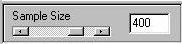 Moving the sliders causes the module to begin simulating normally-distributed
data. The
number of datapoints is determined by the slider in the sample size
panel, which can be between 5 and 500. (Perhaps we should stop the analogy
with Mike and Joe here - it would be rather unfair to make them do 500 tests!)
Moving the sliders causes the module to begin simulating normally-distributed
data. The
number of datapoints is determined by the slider in the sample size
panel, which can be between 5 and 500. (Perhaps we should stop the analogy
with Mike and Joe here - it would be rather unfair to make them do 500 tests!)
Note that if you set all the sliders to zero (which would imply no
variation for either measure) the module will 'compensate' by introducing
a small amount of shared variation. If it did not do this, an error
would occur when calculating the bivariate statistics (it would
imply division by zero). In any case, the concept of covariation is
meaningless if there is no variation in at least one of the measures.
 This module does not show us the individual data points, unlike the
previous two modules (although
we will see a scatter-plot of all the points). Instead, just the
summary statistics are presented, now that we know how they are calculated.
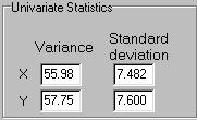
The univariate statistics presented are the variance and the
standard deviation for X and Y.
This module does not show us the individual data points, unlike the
previous two modules (although
we will see a scatter-plot of all the points). Instead, just the
summary statistics are presented, now that we know how they are calculated.
The univariate statistics presented are the variance and the
standard deviation for X and Y.
Note the effect of moving the sliders on these variance estimates. Firstly,
note they that will tend to 'jump around' quite a lot. This is because of
random sampling variation. When we specify the strengths of S1, S2
and C in the panel above, we are specifying the population
parameters. The computer then acts as if it were randomly selected
between 5 and 500 (however many as specified) individuals from this
population. So, on average, we should expect the sample to be
representative of the population.
But we also expect sample-to-sample variation in these estimates. We should also
expect that this sample-to-sample variation is greater if the samples drawn
are of a relatively small size. Confirm this for yourself by making the
sample size smaller. The sliders at the top directly represent the variance
in X and Y attributable to the three causal factors. The estimated sample
variance for X and Y should therefore be close to the sum of these values
(i.e. S1+C for X and S2+C for Y): this will be more likely to be the case
when the sampe size is larger. Note that it is the absolute value of C that
contributes to the variance, however. That is, if S1 were 50 but C
were -25, we should expect the variance of X to be 75 and not 25. This is
because C still generates variation in X - if we are not considering the
relationship between X and Y, then the sign of C is meaningless.
 The sign of C will not be meaningless when considering the bivariate
statistics, however. These statistics are essentially trying to
quantify the extent of the relationship between X and Y. In this
context, they are evaluating the magnitude and sign of the shared cause, C,
relative to the magnitudes of the specific causes, S1 and S2.
The presentation in terms of the shared and nonshared latent variables is
arbitrary, however. See the Appendix for a discussion of the possible
reasons for observing associations between two variables: having a
shared cause is only one of them.
The sign of C will not be meaningless when considering the bivariate
statistics, however. These statistics are essentially trying to
quantify the extent of the relationship between X and Y. In this
context, they are evaluating the magnitude and sign of the shared cause, C,
relative to the magnitudes of the specific causes, S1 and S2.
The presentation in terms of the shared and nonshared latent variables is
arbitrary, however. See the Appendix for a discussion of the possible
reasons for observing associations between two variables: having a
shared cause is only one of them.
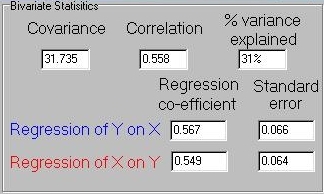
First, we see that the covariance between X and Y has
been calculated. Inside the module, this would have followed exactly the same
procedure we saw in last module. So, again, we find ourselves asking
the question, in this case: so what does a covariance of 31.735
actually tell us about the relationship between X and Y?
The correlation presented in this panel attempts to
answer this, by standardising the covariance with respect to
the variances of X and Y. Specifically, it represents the
covariance divided by the square-root of the product of the
two variances (see the Appendix for a more detailed discussion
of the correlation coefficient). In this case, we see that
31.735 / ( sqrt(55.98*57.75)) = 0.558. Correlations range from
-1 to +1, where +1 represents a perfect positive association,
-1 a perfect negative association and 0 no association. So
a correlation of 0.558 implies a moderate positive association
between X and Y. The square of the correlation represents the
amount of total variance explained by the covariation between the
two traits: in this case, 0.558*0.558 = 0.31.
As explained in the Appendix, the regression coefficients
are a function of the amount of variance in one measure explained by
variation in the other. As such, regression is asymmetrical, in
that we can ask how well X predicts Y as well as how well Y predicts
X. The standard error of the regression coefficent can be
interpreted as a measure of certainty regarding that estimate. If the
standard error is large, it implies that the estimated regression
coefficient may not be representative of the true population value.
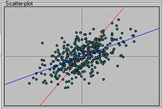
The scatter-plot represents all the points in the sample as well as the
two colour-coded regression slopes.
Exploring the module
Let's use the module to get a feel for the relationship between
these different measures. Firstly, note how moving either of
the two specific slides, S1 or S2, changes the shape of the
bivariate distribution. Increasing S1 will stretch it out
horizontally (for X is represented along the horizontal axis,
traditionally known as the x-axis in any case). This
is because it is introducing variation in X that is not shared
by Y.
Conversely, moving the S2 slider will make the distribution
grow or shrink along the vertical axis. Changing the C slider
has a different effect on the shape of the distribution, and its
effect will be more noticeable when S1 and S2 are quite low. Set
S1 and S2 to about 10 each. If C is at zero, the points should be
clustered in a evenly-shaped little ball in the middle of
the scatter-plot. (Make sure that the sample size is quite high,
over 400 for these effects to be clear).
Note that the variance of both X and Y should be near 10. The
covariance will be very small, however, and the correlation will
be even smaller. The proportion of variance explained should be
virtually zero. The regression slopes should also be virtually zero,
so that the red line will follow vertical axis and the blue line
will follow the horizontal axis. This is because, given that neither
measure tells us anything about the other in this scenario, the
most likely estimate of Y will be the mean of Y, for all values of X.
This is represented by the blue line, the regression slope that predicts
Y given X, which will be virtually flat. Likewise, the red regression
slope predicting X given Y will remain very close to the mean of X at all
points of Y (i.e. will tend to follow the y-axis).
If you then move the C slider to the right slowly, note what happens to
all the statistics and the scatter-plot. Both variances increase, unsurprisingly,
as that is what the slider is doing: adding more variation. But the covariance
will increase also, as will the correlation and all the other statistics. This
is perhaps best represented in the scatter-plot: a clear association between
X and Y will result, in that points that tend to be higher on X also tend to
be higher on Y and vice versa. The two regression lines will begin to converge,
representing this fact.
With C on some high value, set both S1 and S2 to zero and observe what happens.
This state of affairs implies that the only source of variation in both X
and Y is completely shared. Because there is no unique variance in either
X or Y, every individual's score on X would be identical to their score on Y:
thus the straight line on the scatter-plot. In this case, note that the covariance
equals the variance of both measures, and so the correlation is 1. Now move
the C slider to a negative value: the covariance and correlation become
negative, the points align themselves differently on the scatter-plot.
Try reducing the sample size to get a feel for the way in which the
estimates become less consisent. With only a few points, say less than
10, you should be able to see the way in which the regression slopes can be
drastically influenced by just one extreme observation. Note how the
standard errors of the regression coefficients increase too - the implication
of this is that the coefficients would be unlikely to be significantly different
from zero, in a statistical sense.
 Finally, we will consider a case that highlights the difference between
the correlation and regression coefficients. See the following scenario,
where X has a great deal of specific variation (S1=88) but there is no
shared variation (C=0). As mentioned above, the program will
not let a variable have zero variance (i.e S2=0 and C=0); it will
add a very small amount to make the routine run. So think of Y as having
a very small degree of unique variation and no association with X.
Finally, we will consider a case that highlights the difference between
the correlation and regression coefficients. See the following scenario,
where X has a great deal of specific variation (S1=88) but there is no
shared variation (C=0). As mentioned above, the program will
not let a variable have zero variance (i.e S2=0 and C=0); it will
add a very small amount to make the routine run. So think of Y as having
a very small degree of unique variation and no association with X.
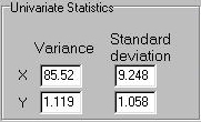 We see these values reflected in the variances of the simulated sample -
X has a relatively large variance, Y has a relatively small variance.
We see these values reflected in the variances of the simulated sample -
X has a relatively large variance, Y has a relatively small variance.
But take a look at the regression slopes, however:
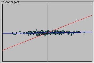
Although we know that X and Y should be unrelated, the regression slope of
X on Y (that is, the red line that plots the expected value of X as
a function of Y) is far from flat. If we look at the actual bivariate
statistics, we see the same pattern:
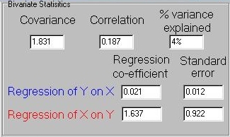
That is, despite the fact that the covariance and correlation are
very small, as expected, as in the regression of Y on X, the
regression of X on Y has a very large coefficient. In this particular
sample there are a reasonable number of individuals, too (approximately
200), which seems to have been enough to estimate the other statistics
accurately. What is going on?
The asymmetry in regression slopes is caused by the
asymmetry in the variances of the two measures and is
unsurprising when you think about it. It is easy to predict
something that does not have very much variation - the mean
will always be a good guess. Therefore, it is easy to predict Y.
It is difficult for Y to predict X however, as X does have a
lot of variation. Because there is such a 'restriction in range' in
Y, relative to X, it is unable to accurately account for variation in X.
This is reflected in the very large standard error for the regression of
X on Y seen here - 0.922 (taken as relative to the magnitude of the
regression slope itself, 1.637). This is why the two regression
slopes tell us slightly different things: whether one
variable predicts another variable better or the other way round is
due to the relative balance of unique variance in each. Note that
if both X and Y have the same amount of unique, 'residual' variance
then both regression slopes will equal the correlation coefficient.
These relations are clearly apparent in the simple equations
that describe the relationship between variance, covariance,
correlation and regression, as described in the Appendix.
Questions
-
-
-
Answers
-
-
-
Please refer to the Appendix for further discussion of this topic.
Site created by S.Purcell, last updated 6.11.2000
|