Behavioural Genetic Interactive Modules
Extremes Analysis OverviewThis module aims to introduce the concept of DF group analysis.Introduction to DeFries-Fulker Extremes AnalysisDeFries-Fulker analysis (DF analysis) is a regression-based method for the analysis of twin data. It was designed particularly for the case of proband-ascertained samples: an example of a non-random sample. This approach ascertains extreme scoring individuals (probands) along with their co-twin. This means that in every twin pair, at least one of the twins will be a high scorer. As a result, standard correlational and model-fitting methods of analysis are no longer entirely appropriate. DF analysis is based on the principle of regression to the mean. To illustrate this, consider the following example: Imagine that we have 1000 individuals and test them on some measure, such as the amount of exercise they had done in the last week. We might expect the following type of frequency distribution chart, where some individuals do lots (at the right-hand-side of the plot), some do none (at the left-hand-side), but most do an intermediate amount (in the middle). If we were to re-test the same individuals a month later,
what would we expect the plot to look like? We have no
reason to believe the mean or variance of the distribution
should have changed at all: on average, nothing special
should have happened to our sample in their exercise
habits. We would expect exactly the same pattern :
However, what if we focused on the group of individuals
who scored very low at the first measurement occasion:
If we were to re-test the same individuals a month later,
what would we expect the plot to look like? We have no
reason to believe the mean or variance of the distribution
should have changed at all: on average, nothing special
should have happened to our sample in their exercise
habits. We would expect exactly the same pattern :
However, what if we focused on the group of individuals
who scored very low at the first measurement occasion:
 Is there any way of predicting what will happen to
the mean of this group at the second measurement
occasion?
The mean at the second occasion of the group who were
extreme at the first occasion will depend on the
underlying correlation between the two occasions.
Imagine the correlation was +1. All individuals would have
exactly the same score at the second time as they had
for the first time. The implication of this is that the
extreme group would continue to be equally extreme at
the second occasion.
Is there any way of predicting what will happen to
the mean of this group at the second measurement
occasion?
The mean at the second occasion of the group who were
extreme at the first occasion will depend on the
underlying correlation between the two occasions.
Imagine the correlation was +1. All individuals would have
exactly the same score at the second time as they had
for the first time. The implication of this is that the
extreme group would continue to be equally extreme at
the second occasion.
The Module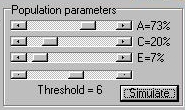 The module simulates a population of 20,000
individuals (5000 MZ pairs and 5000 DZ pairs) according
to the population parameters specified in the panel, as shown
to the right. As well as using the sliders to determine
the relative balance of additive genetic, shared environmental
and nonshared environmental variance for this
trait (A, C and E), we also have to specify a threshold
that will be used to select probands.
The module simulates a population of 20,000
individuals (5000 MZ pairs and 5000 DZ pairs) according
to the population parameters specified in the panel, as shown
to the right. As well as using the sliders to determine
the relative balance of additive genetic, shared environmental
and nonshared environmental variance for this
trait (A, C and E), we also have to specify a threshold
that will be used to select probands.
After simulating the twin population, the module selects the co-twins of probands and plots their scores, separately for MZ and DZ co-twins. The co-twin means are also calculated and plotted on the axes, also. Here is the MZ co-twin distribution. 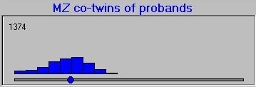 And here is the DZ co-twin distribution.
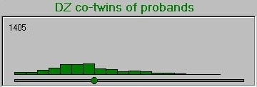
As can be seen from these graphs, the DZ co-twins score higher on average than the MZ co-twins. This represents the differential regression to the mean between MZ and DZ co-twins, that reflects the difference in correlations between MZ and DZ co-twins.
The DF analysis has done a good job here. In this instance, the data were simulated under:
Exploring the moduleTry experimenting with different thresholds and different values for A, C and E in order to see how the MZ and DZ co-twin means reflect these components of variance. For example, notice however both co-twin means regress back to near the population mean when then trait is predominantly determined by nonshared environmental sources of variation.Regression modelTypically DF analysis is performed within a linear regression model. The heart of it is embodied above, however: the comparison of co-twin means. The regression estimates the same quantities but also allows for confidence intervals to be put around the estimates in a very straight-forward manner, using standard statistical packages such as SPSS. See the Appendix and Box 8.1 of the Behavioral Genetics text for further explanation of DF analysis.Heterogeneous PopulationsBut what if DF analysis of extreme probands and their co-twins gives significantly different results to standard ACE analyses for the same trait in similar populations? In this simulation we know that we have simulated a homogeneous population, so the DF estimates should always mirror the population parameters, give or take sampling error. The population is homogeneous in the sense that the population parameters describe the sample equally well at any point along the distribution. It might be that there is 'something special' about the individuals with extreme scores that might represent a different aetiology compared to the unselected population acting in these individuals, however. In this case, we might expect DF analysis to reflect this difference, relative to analysis of variation in the trait throughout the normal range. Such 'special' factors might include rare genes of major effect, certain strong epistatic or gene by environmental effects, or admixed populations. Such factors might imply that the causes of disability, for example, (as indexed by proband status) are quantitatively or qualitatively different from the causes of normal variation (as indexed by standard analysis of individual differences).Site created by S.Purcell, last updated 13.11.2000 |
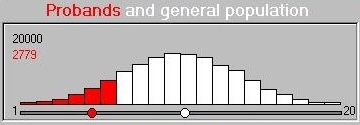 The module simulates a trait that ranges between 1 and
20: the threshold is expressed in the raw-units of the
trait. All individuals scoring at the threshold or lower
become probands. Here we see the distribution of the
all individuals' scores. That is, both twins in a
pair are plotted and so both can become probands if their
scores are both below threshold. Both twins will also be co-twins
in this case. This is called double-entry
and has to be statistically corrected for when estimating
the significance of a DF result (as some individuals are
essentially counted twice) but it does not affect the
ideas we are dealing with here in any way.
The module simulates a trait that ranges between 1 and
20: the threshold is expressed in the raw-units of the
trait. All individuals scoring at the threshold or lower
become probands. Here we see the distribution of the
all individuals' scores. That is, both twins in a
pair are plotted and so both can become probands if their
scores are both below threshold. Both twins will also be co-twins
in this case. This is called double-entry
and has to be statistically corrected for when estimating
the significance of a DF result (as some individuals are
essentially counted twice) but it does not affect the
ideas we are dealing with here in any way.
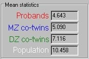 These means are summarised in the panel, shown to the
right. As expected, the proband mean is the lowest, the
MZ co-twin mean the next lowest, the DZ co-twin mean
next and the population mean last.
These means are summarised in the panel, shown to the
right. As expected, the proband mean is the lowest, the
MZ co-twin mean the next lowest, the DZ co-twin mean
next and the population mean last. 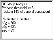 If we transform these means in the manner described
above we arrive at the DF analysis estimates for
A, C and E. This panel also tells you what percentage
of the population were selected as probands for the
specific threshold used.
If we transform these means in the manner described
above we arrive at the DF analysis estimates for
A, C and E. This panel also tells you what percentage
of the population were selected as probands for the
specific threshold used.