Behavioural Genetic Interactive Modules
 Model-fitting to Twin Data : 1OverviewThis module provides an opportunity to explore model-fitting in the context of the quantitative genetic models that are typically applied to twin data. As described in the Appendix, such models decompose the variance of a trait into additive genetic, shared environmental and nonshared environmental components on the basis of the trait covariance observed for identical and non-identical twins.Tutorial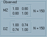 The data to which we will be fitting models are
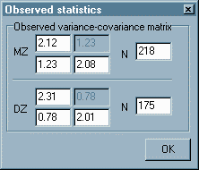
two variance-covariance matrices. These are shown in the top
right panel of the module, labelled Observed. As mentioned
in the Matrices section of the Appendix, variance-covariance
matrices are square, symmetrical matrices containing variances
along the diagonal elements (for, in this case, each twin) and
covariances in the off-diagonal elements.
Although by default the observed variances are all set to exactly 1, these are not correlation matrices – these values were merely chosen for ease of presentation. Technically, if these matrices were necessarily correlation matrices, then the fit-function (which assumes these are covariance matrices, i.e. not standardized) would be biased, although we will ignore this in some examples.
As mentioned, there are two matrices in
this panel – one for all the MZ twins in the sample and
one for all the DZ twins in the sample. The sample size, N,
for each group is written beside each matrix (150 by default).
These observed variances and covariances would be what researchers
calculates, in a package such as SPSS or Stata, from the raw
data they have collected. In this module, the different observed
statistics can be entered by clicking on the
As mentioned in the Appendix, we cannot estimate additive and dominance genetic components at the same time as shared and nonshared environmental components if we only have twin data. The models we will consider in this module are therefore restricted to those that are nested in the ACE model and are commonly evaluated.
One advantage of working with the variance components in this case is that they sum in a straightforward manner to produce the expected variance-covariance matrices. These are displayed in the Expected panel and are a function of the parameter values. How these expectations are calculated is described in the Appendix. Note that all expected variance elements are simply the sum of all the parameters in the model; the expected MZ covariance equals the additive genetic variance plus the shared environmental variance (assuming that both, or either, are estimated, that is, they are not fixed to zero); the expected DZ covariance equals half the additive genetic variance plus the shared environmental variance.
The important thing to remember for now
is that the fit-function is essentially a measure of how closely
the expected variances-covariance matrices match the observed
ones. Smaller values of this statistic indicate a closer fit
– a value of 0 represents a perfect fit. This statistic
is also dependent on the sample sizes. As this particular fit-function
is actually a
Now try moving one of the sliders. Click on the slider in the A box of the Model parameters panel and move it up and down slightly. Notice that several things change as a result of a changing the parameter value of the additive genetic component. First, note that the expected variance-covariance matrices change. The expected variances will increase (becoming greater than 1) and the covariances will also increase as the A slider is moved upwards. Note that the MZ covariance increases at a faster rate than the DZ covariance.
Second, some figures will have appeared in the Model fit statistics panel, for the fit-function (and p value) that is associated with the particular expected variances and covariances that are, in turn, associated with particular values for the three parameters, A, C and E. The two red bars in the Model fit statistics panel represent graphically the current fit-function (the height of the left bar) and the best (i.e. lowest) yet obtained for that particular model (i.e. ACE, AE, CE or E).
It is the behavior of the fit-function with respect to different values for the parameters that is used to estimate the most likely true values for these parameters, given the data. That is, if all different permutations of parameter values were tried, then the set of values which produced the smallest fit-function would form the maximum likelihood estimates of these parameters.
Experiment moving the three sliders up and down. The aim is to find the values for these three parameters that are most likely to be true given the observed statistics. That is, the aim is to get the red bars as short as possible. You can look at the expected variance-covariance matrices also, to provide an indication as to whether to increase or decrease any one parameter. This process is normally called optimization or minimization and is what programs such as Mx and LISREL do automatically. With more complex models, it would soon become very difficult to be reasonably certain that you had in fact found the best-fitting parameter estimates.
For the default observed variance-covariance matrices in this module, it is possible to find a unique set of values that gives a perfect fit between the expected and observed statistics. This perfect fit translates into a fit-function of zero, as mentioned. If we pretend that the observed values are in fact twin correlations, we know that the heritability is twice the difference; the proportion of variance attributable to the shared environment is the MZ correlation minus the heritability; the proportion of variance attributable to the nonshared environment is 1 minus the MZ correlation (see Appendix for details).
If you have not already found this out by experimentation, set the three parameters accordingly: that is, 0.60, 0.20 and 0.20 respectively (given "correlations" of 0.80 and 0.50). Note that this will give a fit-function of exactly zero because the expected variances and covariances will be identical to the observed values. No other values will give as good a fit for these data.
But now we turn to the second question: we have found the best-fitting parameter values for this model, but is this the best-fitting model? Select the AE model from the Model panel and repeat the process, trying to minimize the fit-function. With a bit of experimentation you should find that 0.77 for A and 0.19 for E give the lowest achievable fit for this model, with a value of 2.645.
Now, clearly the AE model doesn’t fit as well as the ACE model. This is hardly surprising given that the AE model is just a nested submodel of the ACE model and we know that the maximum likelihood estimate of C wasn’t exactly zero. However, it is natural to ask whether or not this reduction in fit is significant or not. If the fit of the simpler, nested model is not significantly worse than that of the full model, we naturally favour the simpler model as that which provides a more parsimonious explanation of the observed data.
A note on the presentation of p values in this module: "p < 0.10" actually does imply "p > 0.5" as the value given will always be the lowest possible from the following : <0.01, <0.05, <0.10, <0.30, <0.50, <0.70 and <0.90.
Repeating this for the CE model, you will find that the best-fit parameter estimates lead to a significant reduction in fit in comparison to the ACE model. Also, the CE model does not fit the data well in absolute terms either, as the p value associated with the fit-function of the model at the best-fit parameter values is highly significant. You will also see that the E model fits horrendously (which is unsurprising given the substantial observed covariances). Further exploration
Remember that variance-covariance matrices must conform to certain rules. If they do not the module will probably give an error message as it might, for example, end up trying to divide a number by zero if the observed covariance matrices are not properly specified. For a univariate case, all variances must be greater than zero and all covariances not greater than the variances. In the case of twin model fitting, the ACE model will not properly fit if the DZ covariance is greater than the MZ covariance.
Likewise, the sample sizes specified must be 2 or more - any less and the sample variances would not have been able to be calculated in any place.
Note that, unlike the default values, the variance need not be 1 and it need not be exactly the same for all four elements. This is what would happen in a realistic scenario due to sampling fluctuations. However, as one of the assumptions of the models we are fitting is equality of variance across all individuals (i.e. the four variance elements of the expected variance-covariance matrix will always be identical) then it is unlikely that any of these models will achieve a satisfactory fit is the differences amongst observed variances are too large. Indeed, large variance differences in real samples might suggest some sort of sampling, or ascertainment bias. This would certainly be true if the variance differs greatly within zygosity (e.g. MZ twin 1 versus MZ twin 2). If the variance differs between zygosity group, this might suggest possible complex effects such as certain forms of sibling interaction (where the phenotypic value of an individual is directly influenced by his or her co-twin's phenotype).
Note that the scale of the sliders in the Model parameters panel is automatically scaled to the highest observed variance when new observed statistics are entered.
Try entering different values for the variances, covariances and sample size to get a feel for the power of the classical twin design to detect the aetiological factors that contribute to individual differences in a trait. The questions below provide some exercises that use the module to gain some insight into issues of effect size and sample size. QuestionsQuestion 1. A researcher measures a certain trait in 250 MZ and 280 DZ twins and observes the following variances and covariances for MZ and DZ twins:
Use the module to analyse these data. Which is the best-fitting model? What are the best-fit parameter estimates for this model? What does this tell us about the aetiology of the trait?
Question 2. If a typical trait encountered in behavioural genetic research might be expected to show a roughly 2 :1 :1 ratio of additive genetic, shared environmental and nonshared environmental components, then, using the module, what seems to be the minimum number of MZ and DZ twin pairs needed to detect i) additive genetic and ii) shared environmental effects? (Assume equal number of MZ and DZ pairs).
Question 3. Use the module to see whether the twin method is biased in favour of detecting genetic influence over shared environmental influence, or vice versa. For example, if the A and C variance components are equal, do the AE and CE models tend to be equivalent in terms of fit relative to the full model?
Answers
Answer 1. The ACE model fits this data: there
is a nonsignificant (p>0.70)
Note that these three parameters add up to 3.15, which is close to the average observed variance (notice that the diagonal elements of the expected variance-covariance matrices are 3.15). The expected covariances for MZ and DZ twins are close but not exact - the expected MZ covariance is a little lower than the observed (1.65 compared to 1.76) whilst the expected DZ covariance is a little higher (0.93
The AE model also fits the data,
with a nonsignificant
The difference in the
The CE model does not provide an adequate fit to the data. The fit-function is 12.625 at the best-fit parameter values of 1.29 and 1.92 for C and E respectively. Likewise, the E model fails to be a realistic model for the observed data.
Reviewing the analyses, we see that both the ACE and AE models fit the data well. However, because the AE model does not fit significantly worse than the ACE model, we reject the ACE model in favour of the simpler, more parsimonious AE model. This suggests that the shared environment does not play a significant role for this trait in this sample. The best-fit parameter values suggest that 40% of the individual differences for this trait can be attributed to genetic factors (1.29 / (1.29 + 1.92) = 0.4), the remaining 60% can be attributed to environmental effects that are not shared between twins (1.92 / (1.29 + 1.92) = 0.6).
Answer 2. If a trait showed a 2 : 1 : 1 ratio of additive genetic, shared environmental and nonsharted environmental influences then we would expect to observe an MZ twin correlation of 0.75 and a DZ twin correlation of 0.50. That is, additive genetic variance accounts for 50% of variation in this trait, the shared environment accounts for 25% and the nonshared environmental accounts for the remaining 25%. If we imagined a trait with unit variance, then the covariance between MZ twins is the additive genetic variance plus the shared environmental variance, which is 0.50 plus 0.25 equals 0.75. For DZ twins, the covariance would be half the additive genetic influence plus the shared environmental influence which is 0.50/2 plus 0.25 equals 0.50.
Input these values as Observed statistics (i.e. variances of 1, and covariances of 0.75 and 0.50 for MZ and DZ twins respectively). Set the number of MZ and DZ pairs to a relatively high number, say 750 each. Check that, under the ACE model the best fitting parameter estimates for these data are in fact in the ratio of 2 : 1 : 1 (that is, they should be 0.50, 0.25 and 0.25 for the A, C and E parameters respectively).
When we talk about "detecting an effect" we are referring to the comparison in model fit between a model that estimates a parameter corresponding to that effect and a model that fixes this parameter to zero and doesn't estimate it. For example, if the CE model fits significantly worse that the ACE model then we would conclude that we have detected an effect of additive genetic influence.
Power to detect a certain effect will depend on sample size: we can explore this using the module. We have set the sample size to 750 for both zygosities. Click on the CE model and find the best fitting parameter values for the C and E components (these will be 0.63 and 0.37). Note that the reduction in the chi-squared statistic in comparison to the ACE model (92.931) is significant (p < 0.01). As noted above, this corresponds to "detecting an effect" of additive genetic influence.
Click on the New Observed button and reduce the sample size to 500 MZ twin pairs and 500 DZ twin pairs for the same variance-covariance matrices. Set the sliders to the best fit values for the ACE and CE models (these will be the same as above, of course). Here, however, the reduction in fit is only 61.954, although this is still significant.
By reducing the sample size we can see when the reduction in fit becomes nonsignificant - this represents the point at which we can no longer detect the effect, due to the low sample size.
For N=100 for both zygosities, the reduction in fit is 12.391, which is still significant (p < 0.01). For N=50, the reduction is 6.195, still significant at p < 0.05. For N=25, the reduction is 3.098, which is not significant (p > 0.05).
By gradually increasing the sample sizes, we can determine that at least 31 MZ and 31 DZ twin pairs are necessary to detect an additive genetic effect of this magnitude.
By a similar logic, but comparing the reduction in fit of the AE model in comparison to the ACE model, the minimum number of twin pairs need to detect the shared environmental effect can be determined. The best fit parameter estimates for the CE model are 0.74 and 0.24. It turns out that 152 pairs of each zygosity are needed in order to detect a shared environmental effect of this magnitude.
Note that the power to detect an effect will also depend on the magnitude of the true value of other parameters in the model. For example, a different number of twin pairs might be needed to detect a shared environmental effect that accounts for one quarter of trait variance if there were no additive genetic effects for that trait.
Here we have constrained the number of MZ twins to equal the number of DZ twins. You could explore the relative impact of each type by letting these values differ. Of course, it is not only the absolute number of twins that matter - 100 MZ twins and 100 DZ twins will provide more information than 190 MZ twins and 10 DZ twins.
Answer 3. We can use the modules to investigate the relative reduction in model fit for dropping either the A or the C parameters from the ACE model when additive genetic and shared environmental effects explain equal proportions of the trait variance. As we shall see, there are no consistent biases inherent in the ACE model, although the power to detect additive genetic and shared environmental effects does alter as a function of the sample size and the effect sizes of the three components of variance.
As a first example, imagine that the additive genetic variance and shared environmental variance each accounted for 10% of the trait variance. The expected correlations would be 0.20 for MZ twins and 0.15 for DZ twins. Enter these as the Observed statistics (for any 150 MZ twins, 150 DZ twins) and move the sliders to the best fit estimates for A, C and E under the full ACE model (i.e. 0.1, 0.1 and 0.8). Now select the CE model and find the best fit parameter estimates. The drop in chi-squared relative to the full model (given in the bottom right panel) is a measure of the power to detect the additive genetic effect accounting for 10% of the variance. In this case, it is a nonsignificant drop, so we would not be able to detect it. Repeating this procedure for different values of A and C we find the following pattern. At low levels, the power to detect additive genetic effects and shared environmental effects is roughly equal (with shared environmental effects being marginally favoured, i.e. the figures slightly higher under the Drop C column). However, for large effects (the last row of the table) the model is biased for detecting additive genetic effects.
Note : sample size is 150 MZ twin pairs, 150 DZ twin pairs
The picture is complicated by a number of factors that make generalization difficult. Firstly, the power to detect a certain effect is dependent not just on the sample size and the magnitude of that effect, but also on the balance of other effects. For example, if additive genetic effects account for 20% of the variance but the remaining 80% is entirely accounted for by nonshared environmental effects then the reduction in model fit when fixing A to zero is greater than 1.461 for 150 pairs of each zygosity (i.e. the second row in the table above). That is:
Finally, sample size will have an effect on the power to detect all these effects. If the number of MZ and DZ twins is always held equal to each other, then the relative balance of the power to detect A versus C does not alter. However, having many more MZ twins increases the power to detect additive genetic effects; having many more DZ twins increases the power to detect shared environmental effects.
Note : values for one fixed set of parameter values: 2 : 2 : 1 ratio for A : C : E.
In conclusion, we have discovered that the power to detect additive genetic and shared environmental effects depends on a number of factors : the absolute and relative magnitudes of the A, C and E parameters (i.e. the twin correlations) as well as the absolute and relative number of the MZ and DZ twin pairs in the analysis. Site created by S.Purcell, last updated 6.11.2000 |
||||||||||||||||||||||||||||||||||||||||||||||||||||||||||||||||||||||||||||||||||||||
 The
Model panel is used to specify which model we are fitting
to the observed data. By default, the module evaluates the ACE
model: that is, all three parameters (additive genetic, shared
and nonshared environmental factors) are allowed to vary freely.
In the nested submodels, AE, CE and E, one
or more of these parameters is fixed to zero. By clicking on
the different models, you can see how the fixed parameters disappear
from the Model parameters box to the side. For example,
if you select to fit the CE model, then the A slider
disappears from the adjacent panel, representing the fact that
it is fixed to zero (equivalent to saying that additive genetic
factors do not play any significant role in the aetiology of the
trait).
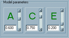 The
sliders in the Model parameters panel represent the values
that the model parameters will take. Note: in this module,
the values are unstandardised variance components and
not standardised path coefficients. That is, the values
these parameters will not necessarily sum to 1. The distinction
between variance components and path coefficients is covered
in the Appendix and we will not dwell on it here, except to reiterate
that these values represent the s 2A, s
2C, s 2E as denoted
in the Appendix.
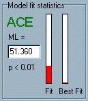 Given
our sample-based observed statistics and our model-dependent
expected statistics we derive an index of fit that can tell us
firstly about the likelihood of different parameter values for
any one model and, secondly, about the likelihood of different
models. The panel Model fit statistics displays the maximum
likelihood fit-function. Details for how this is calculated can
be found in the Mx documentation and standard texts on
model-fitting such as Loehlin’s Latent Variable Models
(see Reading Lists).
 statistic, it is easy to attach
a certain significance value (i.e. p value). This value
is also shown in this panel. Remember that as a small value of
the fit-function indicates a good fit, we ideally want to find
values for the parameters that generate a non-significant
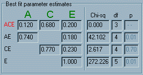 The
panel Best fit parameter estimates keeps track of the
best-fitting parameter values discovered so far. That
is, the "chi-sq" value corresponds to the height of
the right-hand red bar in the Model fit statistics panel.
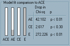 The
bottom right panel, Model fit comparison to ACE, gives
us information about the difference in fit between the full ACE
model and the three nested submodels. As explained in the Appendix,
testing the difference in the fit (i.e. 2.645 – 0.000) we
find that the difference is not significant (i.e. p <
0.30).
 Now
that the basics of this module have been explained, you can use
it to explore some of the more subtle properties of model-fitting
to twin data. Click on the