NAP portal
A beta-version of our NSRR Automated Pipeline (NAP) that hosts the Sleep-EDF Expanded dataset is available for testing at the URL below:
NAP URL: http://remnrem.net/nap/
Info
The fully operational version (that allows external users to upload their own EDFs for processing and visualization) is not yet public. Please contact us if you are interested in beta-testing this particular component of NAP.
Overview
NAP processes and displays sleep signal data, with a focus on EEG signals from whole-night polysomnography.
NAP comprises two main components:
-
a backend processing pipeline for individual sleep studies (EDFs), deriving a set of metrics that describe sleep macro-architecture and EEG micro-architecture
-
a web-based frontend for viewing signals, annotations and any associated derived metrics
NAP has two main entry points:
-
using the NAP frontend to view previously processed cohorts assembled by us (i.e. the Purcell lab/NSRR). Currently, the only public dataset freely accessible via NAP is the Sleep EDF dataset.
-
alternatively, the EDF uploader can be used to upload one's own studies, after which the NAP backend is triggered and the signals along with the NAP-derived metrics can be viewed via the NAP frontend as above. Currently, this option is still being developed and is not open to the public.
Info
NAP is hosted in the AWS cloud and powered by Luna. The frontend viewer uses lunaR and Shiny R packages.
Info
This page is written from the perspective of a user of the NAP frontend; in future posts, we will describe in more detail 1) the steps of the NAP QC process, and 2) notes on how to host your own NAP instance.
NAP backend
Currently, the NAP backend supports the following:
- EDF validation and description
- visualization of signals and any associated annotations
- sleep stage (macro-architecture) metrics
- automated sleep staging
- multitaper spectrograms
- EEG spindle/slow oscillation detection
These procedures are implemented using Luna; in the future, we hope to add further domains of functionality, including respiratory signal analysis.
NAP frontend
Below we step through some of the panels and features of the NAP frontend (using the public Sleep-EDF dataset as an example).
Portal view
The NAP frontend is arranged as below:
Key features are that:
-
the left panel is used to select the cohorts, individuals, channels and/or annotations one is interested in
-
the top panel has various tabs (e.g. NAP, Headers, etc), which bring up various images and/or statistics in the main window area
-
the NAP frontend works mostly one individual (EDF) at a time: that is, all results shown in the tabs are for that selected individual (i.e. whichever EDF is selected in the Samples combo box to the left).
-
one exception to the above principle is the Sample Metrics tab, which gives summary statistics for all individuals in a given cohort
Depending on the exact configuration and context for using NAP, some tabs may not appear (e.g. NAP, Phenotypes, Sample Metrics).
Info
The current example instance of NAP (at http://remnrem.net/nap is pre-populated with the Sleep-EDF cohort only.
Selecting individuals
To select the individual (EDF) to be viewed, use the Samples combo box on the left panel:
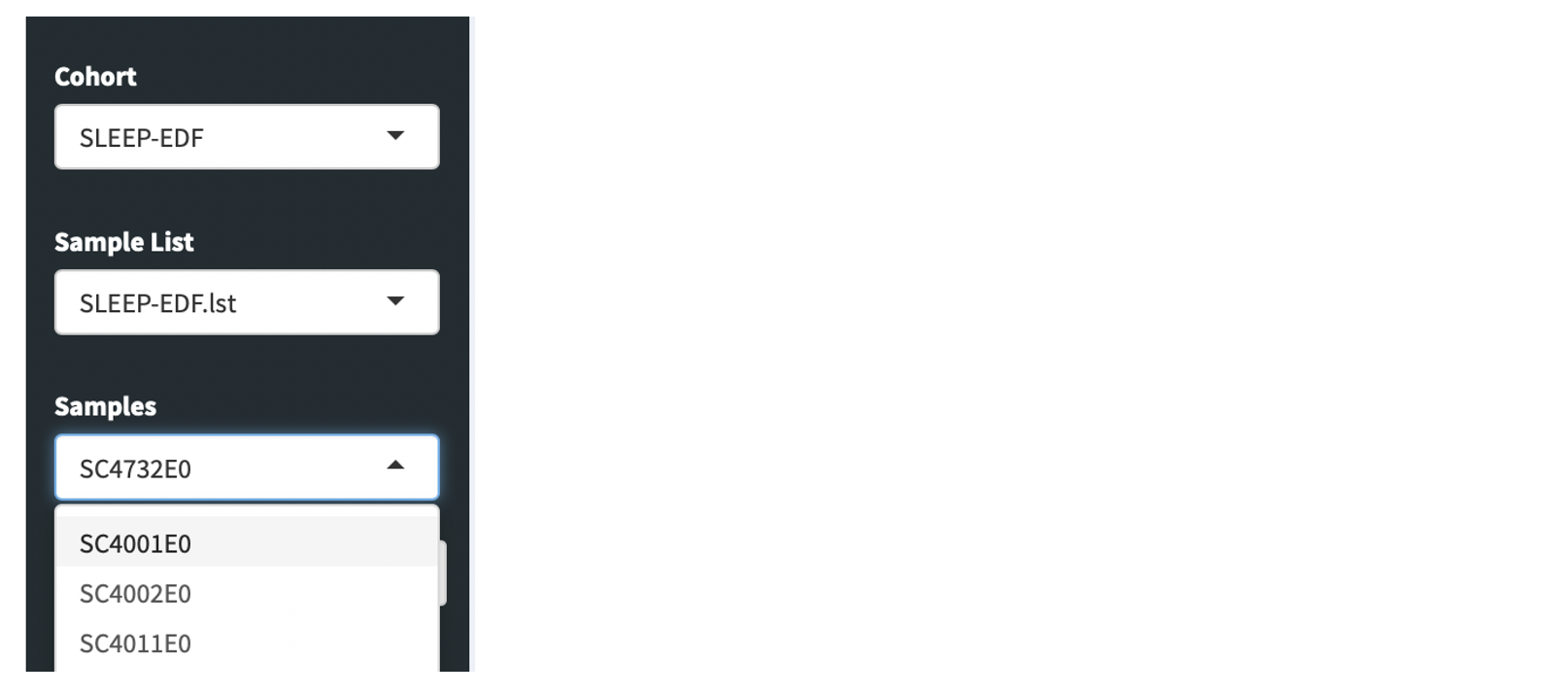
You can either select the individual via the list, or you can also just start typing in the box, and the list will autocomplete with the matching selections.
Tabs
Once an individual is selected, the information on the subsequent tabs will relate to that selected individual. As mentioned above, not all tabs may appear (depending on the configuration of the project, and whether certain fields have been pre-populated, i.e. additional phenotypic information association with a given individual).
The core tabs are shown here, each of which is further described below.

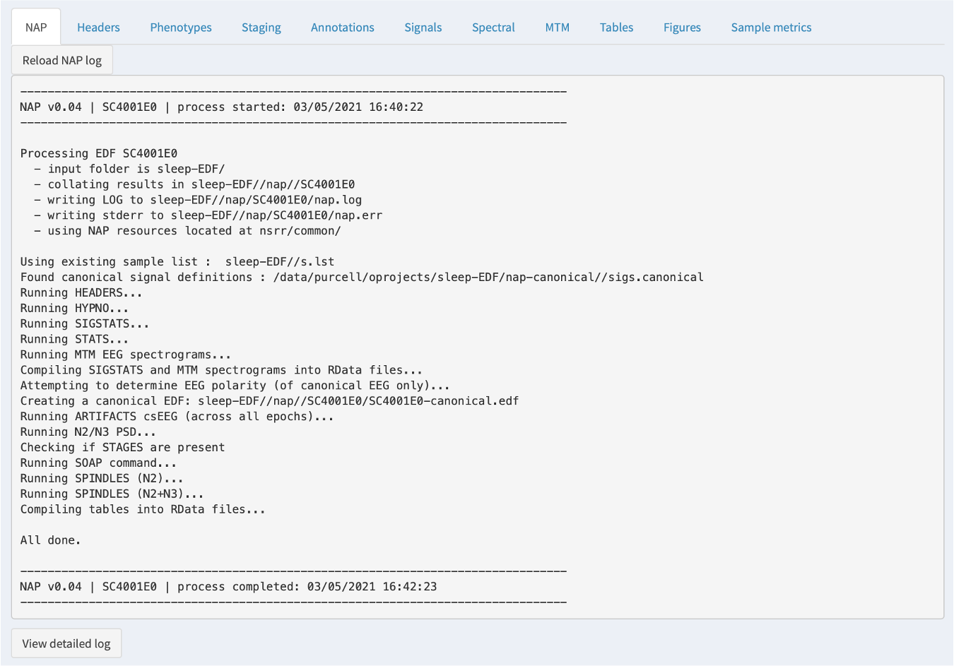
NAP
If the NAP backend has been initiated or previously run, then a NAP tab will show the log information from that process. This is most relevant if something has gone wrong: the information here may be useful in diagnosing the issue. In particular, the bottom of the tab has a View detailed log button: when clicked, this expands a longer log with more detailed error messages.
Info
NAP is nonetheless a work-in-progress: we will be actively working on better diagnosing why a given study failed or not.
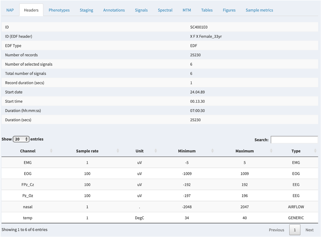
Headers
The Headers tab shows information read directly from the EDF header. Note that the main ID used by NAP is the Luna ID, which may (as in this example) differ from the "internal" ID within the EDF header. It will either be based on a supplied sample list or be based on the filename of the EDF; see here for more information on how Luna structures projects.
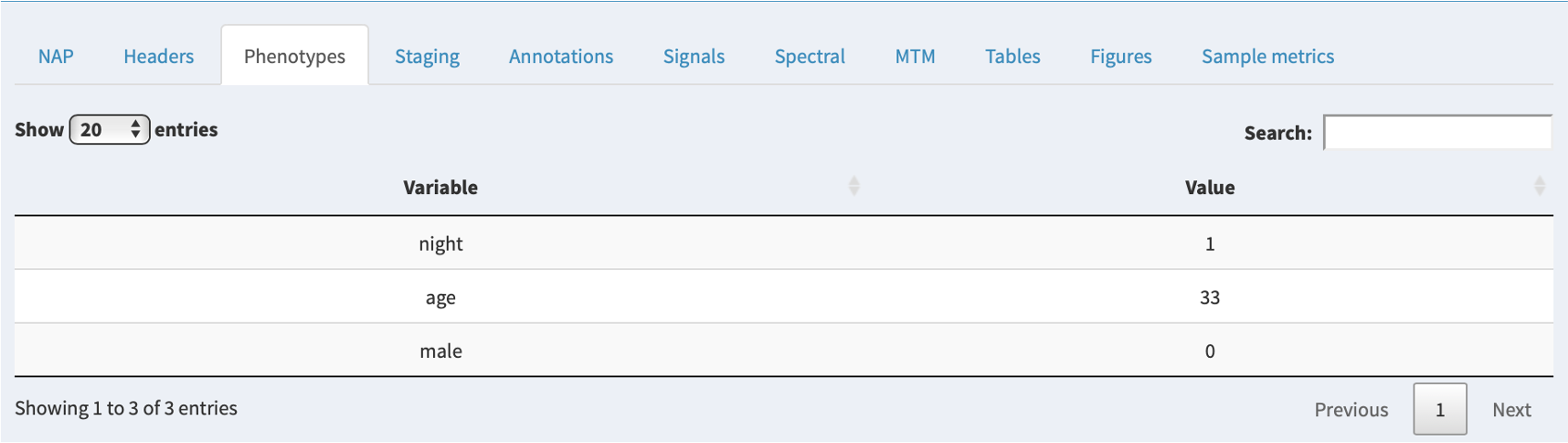
Phenotypes
If additional phenotypic information has been attached to a project, the relevant row for that individual will be shown in this tab. If there are no extra phenoypes, this panel will not show.
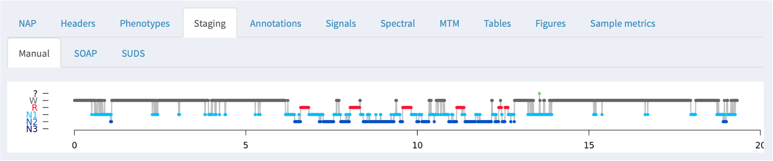
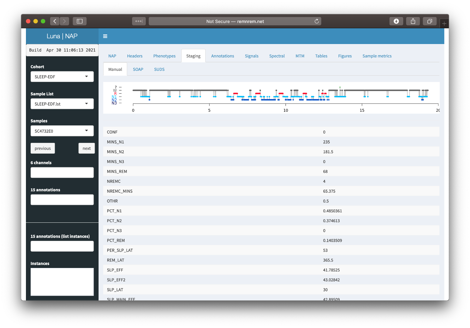
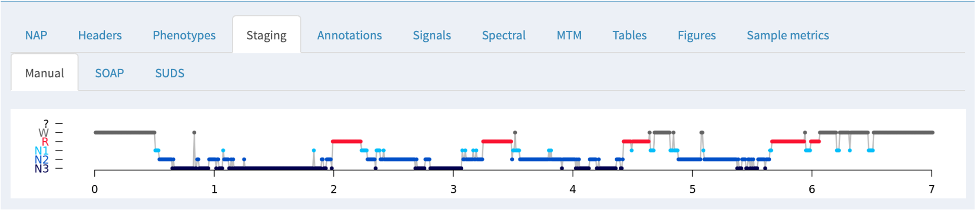
Staging
If NAP detects sleep stage information in an associated annotation file, it will be displayed here, along with the summary statistics obtained from the HYPNO command:
If a canonical EEG (or other signals) have been designated and match the current NAP training data (as will be described in future posts) then NAP will also perform two extra steps:
-
SOAP (Single Observation Accuracies and Probabilities): this fits a model based on the signal data to the observed staging data, trying to spot potential staging errors and/or assess the general consistency of the signals and stages
-
SUDS (Staging Using the Dynamics of Sleep): full prediction of sleep stages based on prior training data (i.e. as one might want if there were no manual staging available)
Describing SOAP and SUDS is beyong the scope of this page: these will soon be described in more detail in the next release of the Luna software and documentation.
In these cases where manual staging was available, both SOAP and SUDS tabs show the original (manual) staging hypnogram at the top (i.e. the same of the Manual tab), and below the model-based/predicted staging. In between, epochs that are discordant between observed and predicted have an orange tick mark; further, epochs that are discordant with respect to the three-way NREM versus REM versus wake classification have a red tick.
Below the hypnograms, the area plot shows the posterior probabilities stacked (i.e. the y-axis represents the probabilty, which sum to 1.0 for each epoch). The amount of each color is therefore proportional to the confidence in that stage assignment.
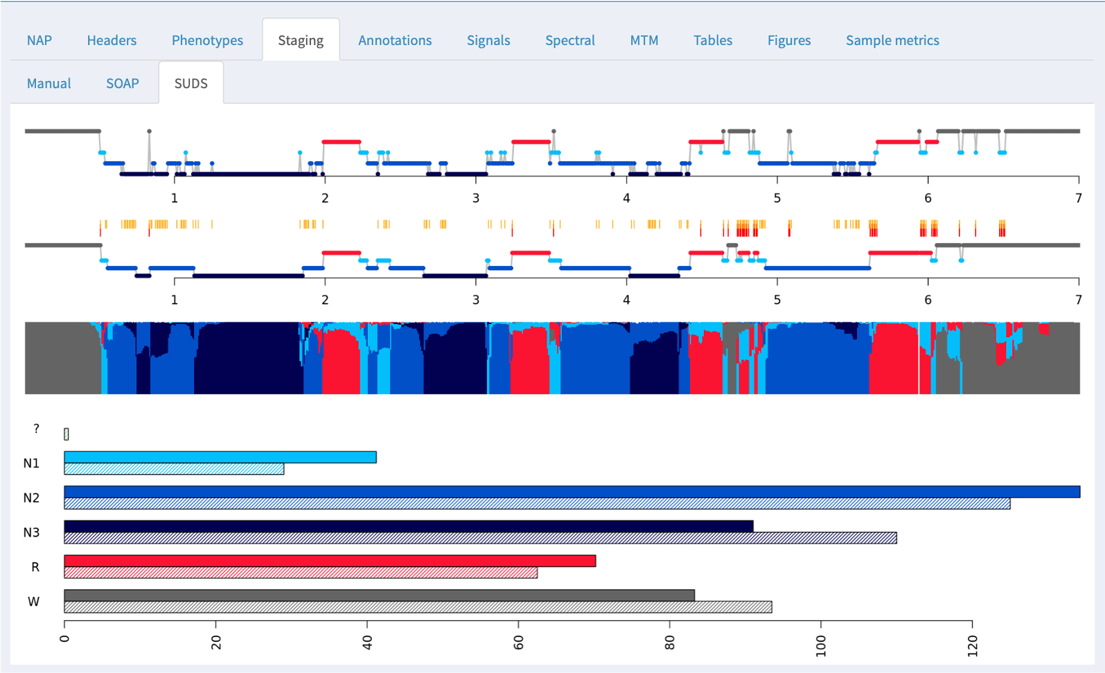
At the bottom of the panel, the bar plots show the estimated (top/solid) and observed (lower/hatched) stage durations in minutes.
Tabular output from SOAP and SUDS is also available in the Tables tab, described below, including the accuracy (ACC) and kappa (K) values.
For this particualr individual (the first individual in the cohort, SC4001E0) staging using the default parameters has done a reasonable job. If you go to the Tables tab (described below) and look at the SUDS group of tables, then select the luna_suds_SUDS table, you will see the accuracy (ACC) and kappa (K) are 0.825 and 0.77, which are comparable to manual staging. (The 3-class values for NR/R/wake classification are higher still: 0.945 and 0.90).
Note
The exact parameterization and training data used for SUDS will greatly impact its performance: the values here are from a default run without extensive tuning. In general, automated staging performs less well for the older individuals in this dataset, but is in most cases quite good. Note that we have removed the extensive leading and trailing wake periods in the Sleep-EDF data prior to populating this NAP instance.
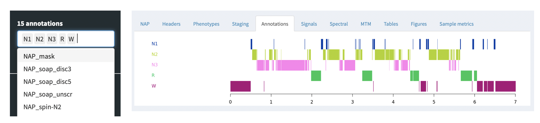
Annotations
Any annotations -- either as generated by the NAP backend, or that
were paired with the original EDF, e.g. via an XML or .annot file, as
described here -- can be viewed
under the Annotations tab. This just shows a box corresponding to
the occurrence of the annotations, for the set of annotations selected
in the left Annotations combo box. All annotations starting with
NAP have been added by the NAP pipeline: as the NAP backend evolves,
we expect a much richer set of annotations to be generated by default.
Signals
The Signals tab allows one to view the raw EDF channel data, showing both selected signals (e.g. EEG) and any selected annotations (i.e. as selected by the Channels and Annotations combo boxes on the left):
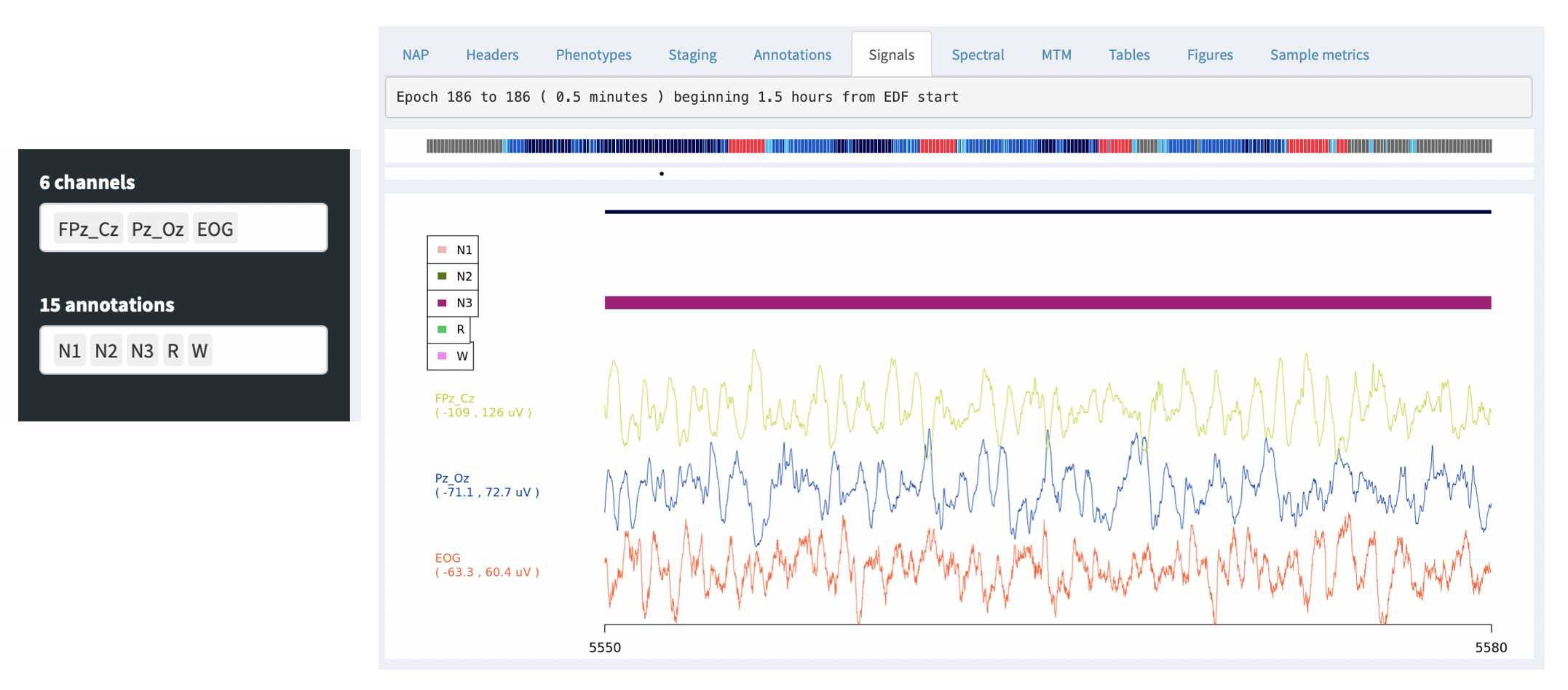
By default, the signal viewer will show a 30 second interval/epoch. You can zoom out by clicking on the hypnogram bar at the top (holding down the mouse button and selecting an interval). If you select a large interval, rather than attemptiong to show the original signal data (i.e. which may be millions of sample points), the viewer will show an epoch-level summary, as below:
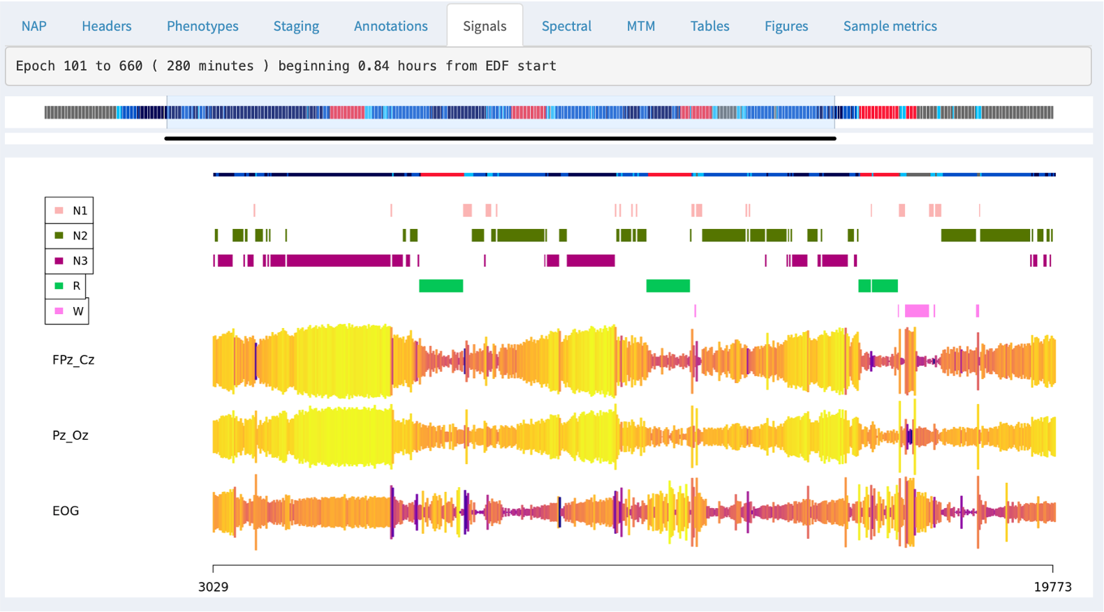
The top of the plot shows the part of the hypnogram that is selected in the top hypnogram, i.e. and so aligns with the zoomed-out signal/annotation data.
For signals with sample rates above 50, NAP will by default show the signal mean amplitude (actually the first Hjorth parameter, activity) as the height of the line; the color of the line represents the second Hjorth parameter, which reflects the frequency of the signal (normalized within channel). These views can be useful for spotting if a signal drops out entirely, or shows major discontinuities over the course of the recording.
For signals with slower sample rates, NAP will instead show the mean of the signal (i.e. as typically those signals will reflect heart rate, temperative, oxygen levels, light, etc - i.e. things where the epoch level average is a meaningful summary, unlike an EEG, EOG, EMG or ECG.
The Signals panel also can use an additional feature of the left
panel: the so-called Annotations (list instances). Whereas the top
Annotations combo box will determine whether or not an annotation is
shown in the display, if you select an annotation in this lower box,
it will then list all instances of that annotation class in the box
below: for example, here showing 490 NAP_spin-N2 instances, which
are spindles detected during N2 sleep by NAP. (In future NAP documentation,
we will enumerate all annotations created by NAP.) Clicking on one of those
instances (or using the cursor keys to move up and down) will make the main signals
viewing panel move to the epoch in which that annotation starts.
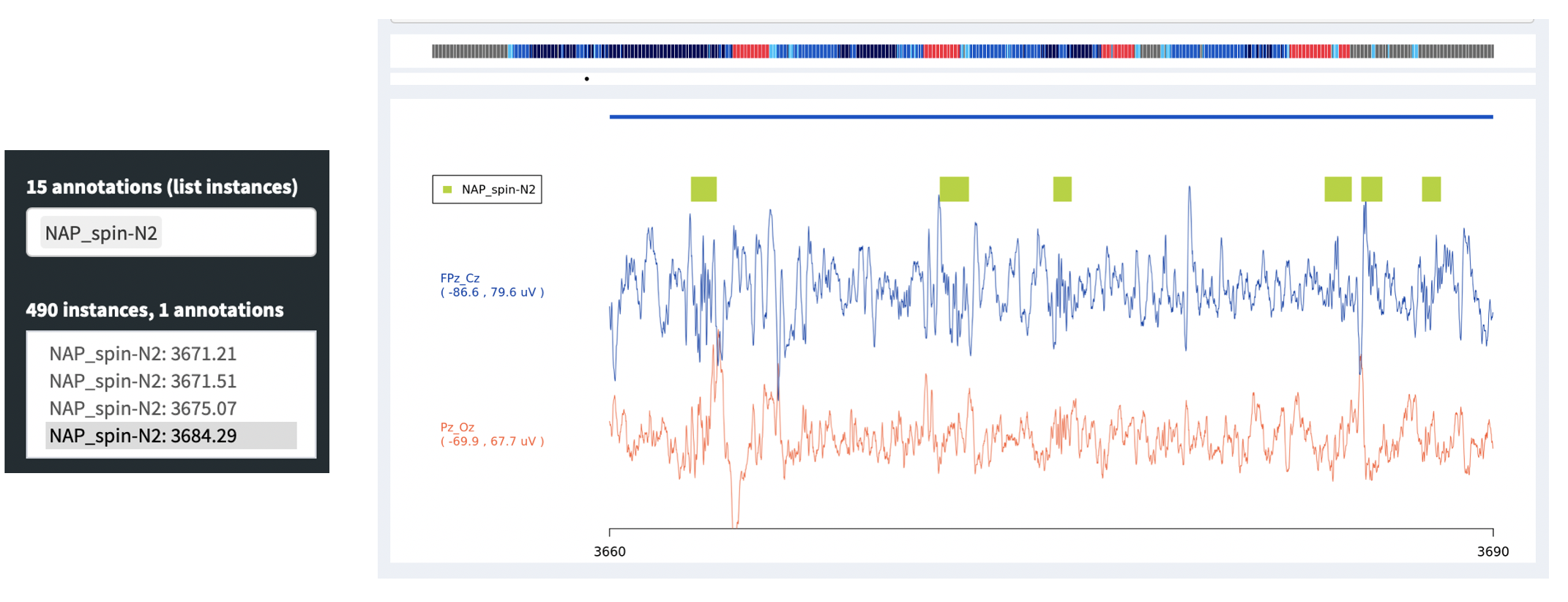
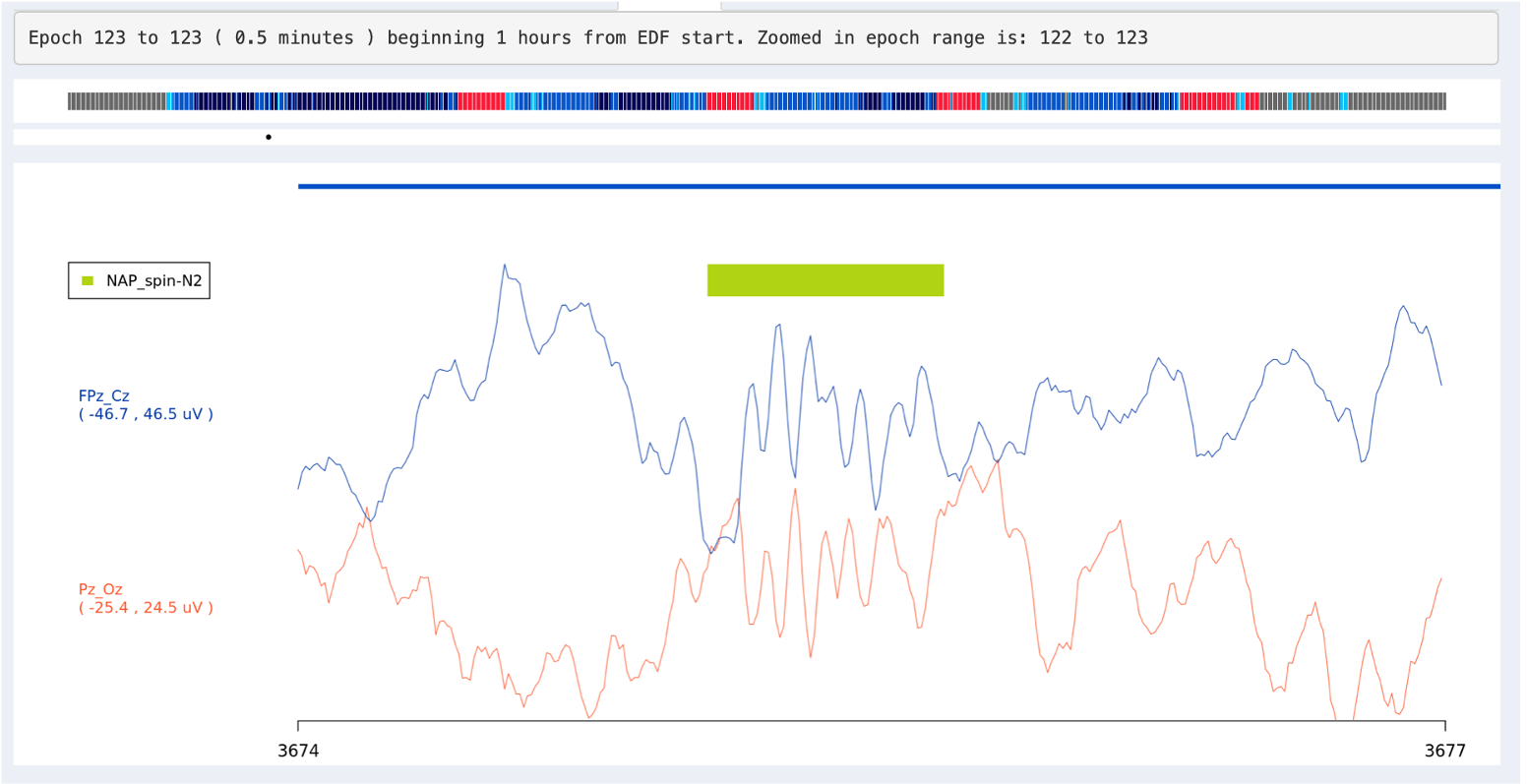
Alternatively, you can click on the inner signal window and select a region to zoom in, i.e. such that the entire window spans only, say, 1 second instead of 30 seconds. To get back to the standard 30-second view, click any signal point on the top hypnogram. In the plot below we've zoomed into a 3-second span (the x-axis of the plot shows seconds elapsed from the start of the EDF), during which a spindle was detected (the green bar).
Warning
The main purpose of NAP is to display the metrics derived from the NAP backend, and try to connect them to the original signal data. That is, the NAP signal viewer is not designed to be a truly flexible, interactive experience, as one might expect, e.g., in a tool for manually scoring sleep studies. There are plenty of other EDF viewing tools for that purpose.
Spectral analysis
For QC purposes, the NAP frontend provides on-the-fly spectral analysis of signals in the Spectral tab, estimating power spectra based on the Welch method (as described here). The slider at the top controls the frequency range shown (which will only go as high as half the sample rate for any given spectrum).
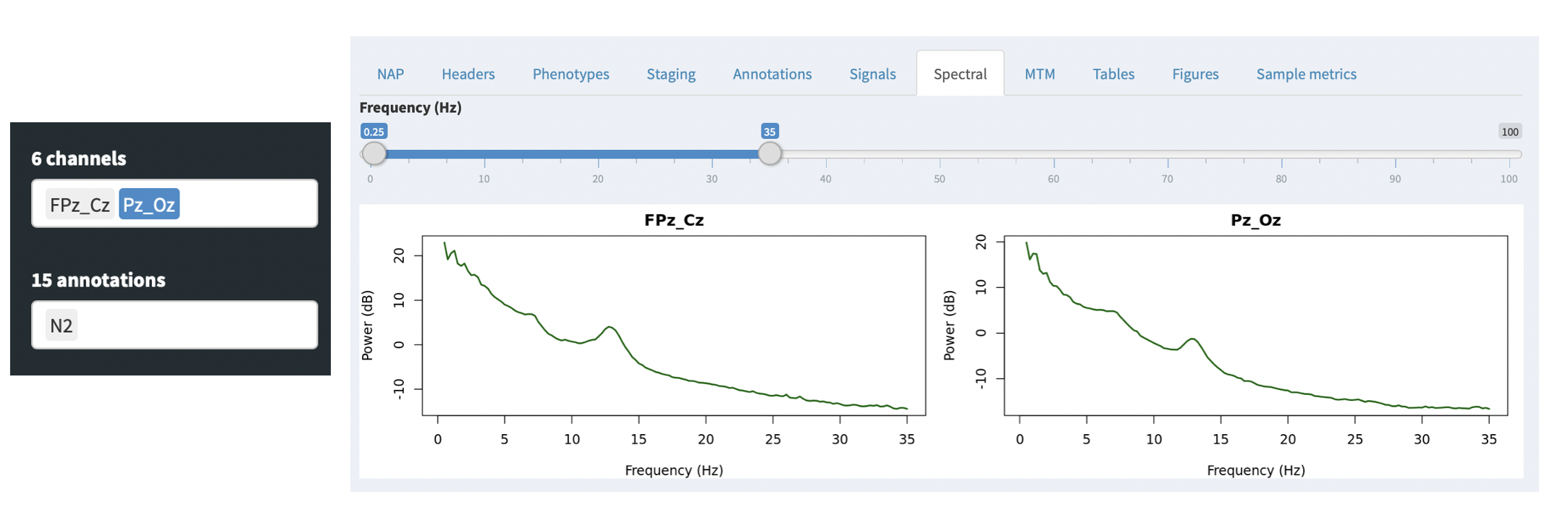
If any annotations are selected (in the leftmost Annotations combo), then these power spectra are calculated only for epochs with those annotations. This provides a quick way, for example, to select only N2 epochs (as in this example) and check that the power spectra look broadly consistent with clean data (i.e. here showing a peak in the sigma/spidle range, but otherwise showing a typical 1/f distribution (plotted here on the log-scale).
Multitaper spectrograms
The NAP backend precomputes multitaper spectrograms for all channels with a sample rate of 50 or more, and shows the images. Unlike the previous Spectral tab, the spectrograms in the MTM tab are fixed (i.e. will not change based on selecting channels and/or annotations).
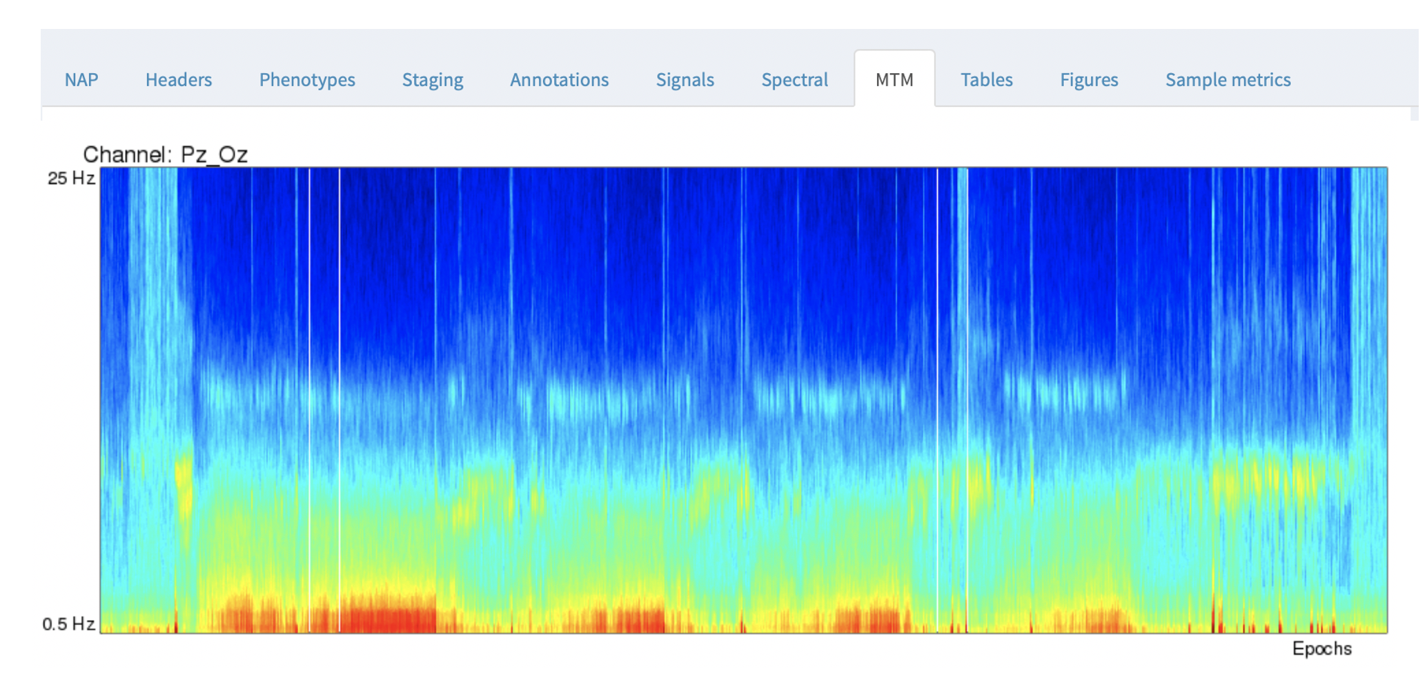
By default, the y-axis is from 0.5 to 25 Hz, the x-axis corresponds to all epochs across the entire recording.
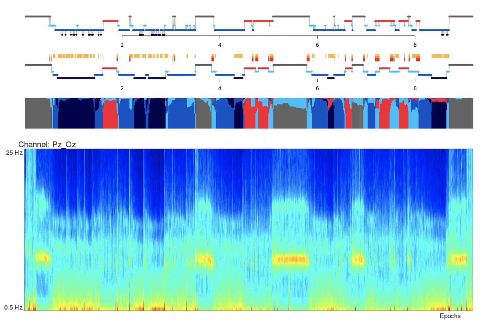
For this example, you can line up the hypnogram (from the Staging tab) and the EEG multitaper spectrograms, and clearly see the correspondence between wake and sleep in the occipital alpha rhythms in the Pz/Oz channel.
Note
TODO: In the future, we may add the default hypnogram to the top of this page, scaled to the same size of the spectrograms.
NAP derived metric tables
If the NAP backend has been run for the study in question, any resultant tabular outputs will be given in the Tables tab.
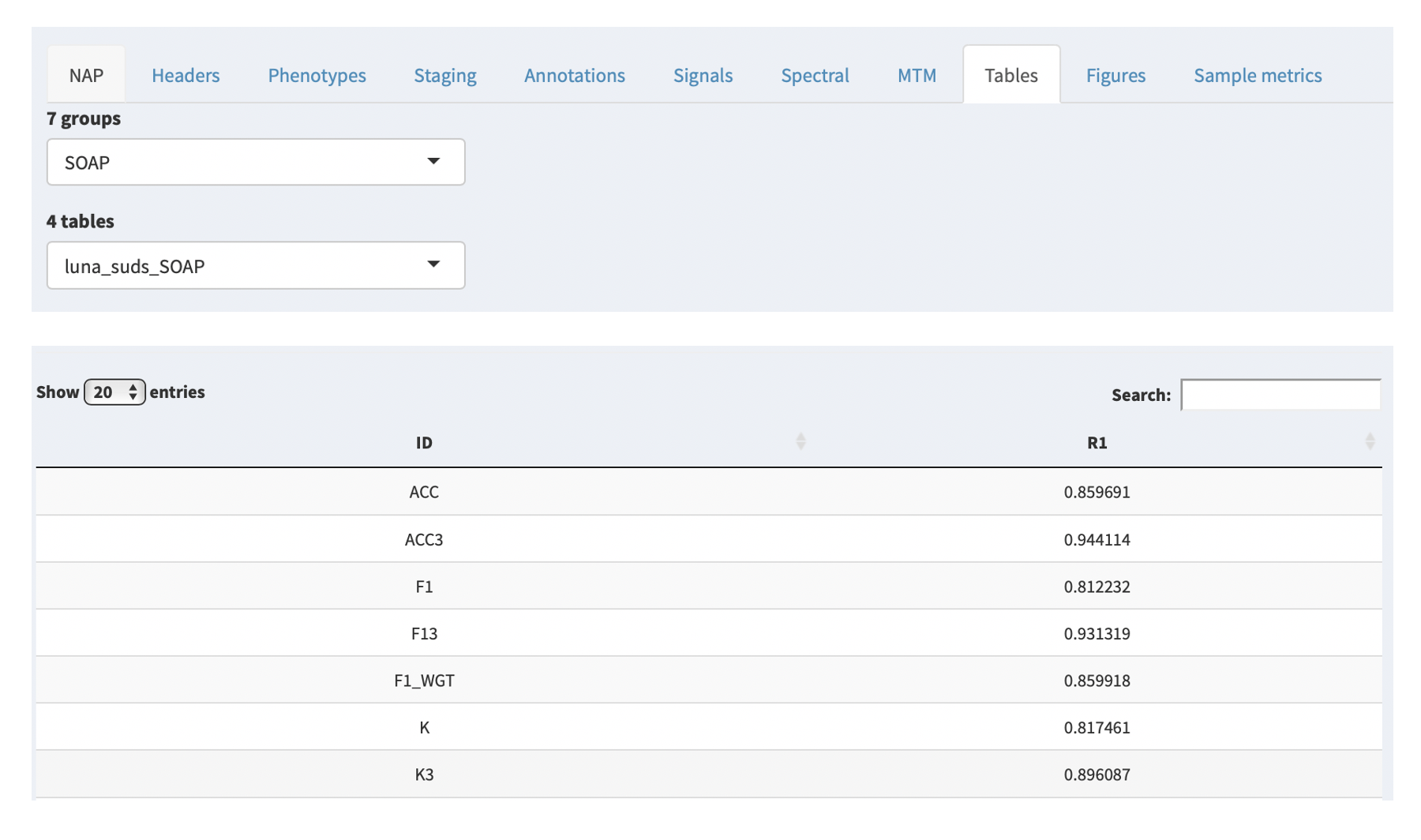
Based on the NAP backend, these are organized by group (i.e. macro-architecture, spindle analysis, etc) and each group contains 1 or more tables. Selecting a table from the second combo box will then display that table below. As the NAP backend evovles, we will add links to describe the sets of metrics computed. As is, these are automatically compiled by the pipline, in the following form:
tool_domain_command{_strata}
In the examples given, the tool is always luna; the domain
corresponds to the broad class of analysis (i.e. here automated
staging, so suds). In this particular case, the command that
generated these tables was the Luna SOAP command. Thus, the table
is called luna_suds_SOAP.
Any further underscore-delimited values indicate that the output is
stratified by that factor: e.g. for the SOAP command there are
additional tables: luna_suds_SOAP_E (which shows epoch-level output,
E) and luna_suds_SOAP_SS (which shows output for each sleep stage,
SS). For all Luna output, these stratifications directly match the factors
and levels in the output of different commands, as extensively described in
the Luna documentation.
The variables in the table (i.e. ACC, ACC3, etc) can be determined by
looking at the documentation for the relevant tool and command.
Note
As mentioned above, these tables are currently programmatrically generated and so have this type of labelling, rather than plain English: in future, we will be adding more decriptive links/titles to each table (along with links to the Luna or other documentation that describes what the particular variables mean).
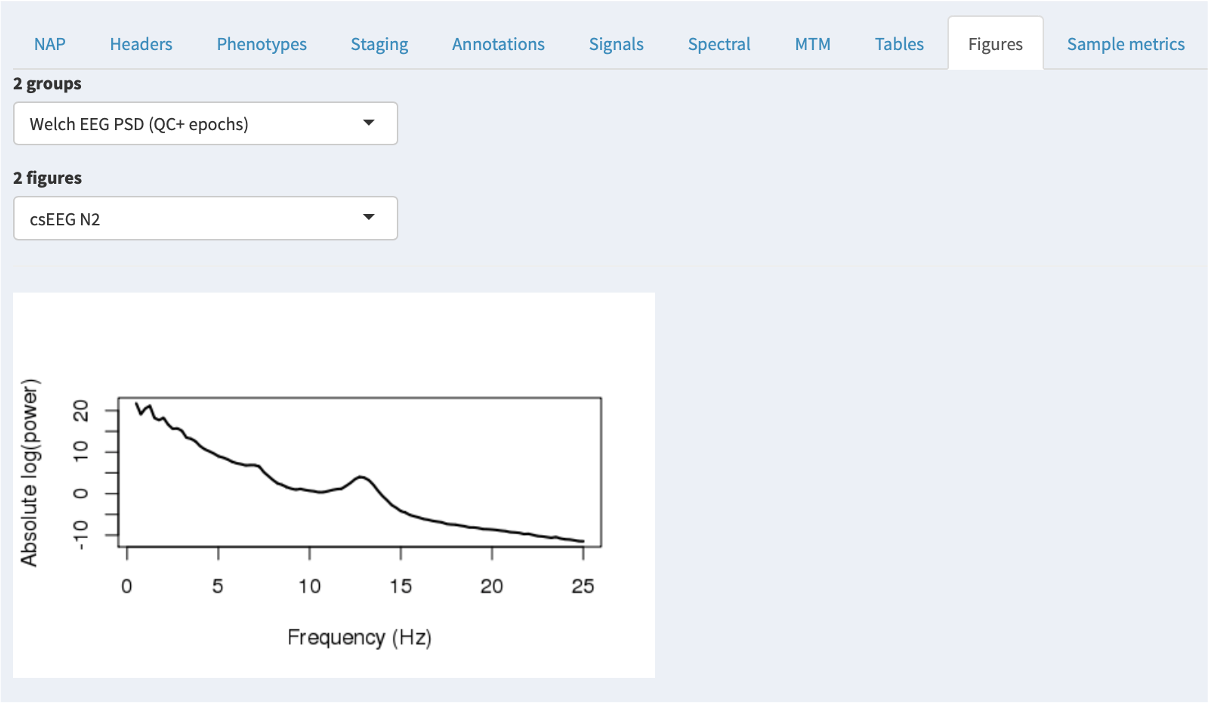
NAP figures
The Figures tab parallels the Tables tab, showing any images generated by the NAP backend instead of tables. Currently, there are only a few images generated, but we expect this to increase over time.
Sample-level derived metrics
Finally, outside of the NAP backend, it is possible to compile one or more sample/cohort-level datasets and attach them to the NAP frontend, in which case they will be displayed via the Sample metrics tab. That is, in contrast to all other tabs/panels, which only show the single, selected individual/EDF, this tab can show information for multiple individuals.
In the example below, there are several groups (here, macro-architecture and micro-architecture), and each group has several tables. Each table then has several variables; selecting a variable will show the distribution of that variable (if it is numeric) in the upper-right plot. The red line indicates where the currently selected individual falls for that variable.
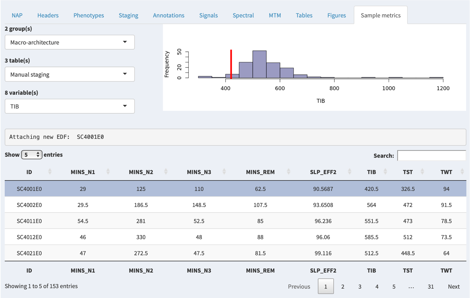
Here we've selected TIB (Time In Bed) and can see that the selected individual (the top gray row, and the red line in the plot) has a relatively low value (420.5 minutes).
Hint
Although in this example, the Sample metrics data happen to have come from the NAP backend, in principle these tables could be any type of data (i.e. genetic, imaging, questinnaire, etc). That is, these are specified as R data frames, that if found in the folder, are automatically uploaded. The data here are linked to the sleep signal data only by the ID, otherwise these values are completely independent of NAP per se. This means that the Sample metrics data could contain individuals not even present in the main cohort, if so desired.
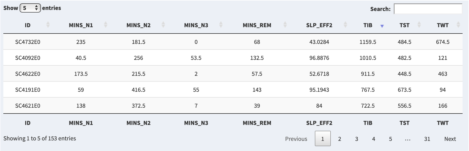
It is possible to sort the table by either ascending or descending order of a given metric by clicking on that column header: e.g. here clicking on the TIB column, we now see the top row is for SC4732E0:
If you click on the row in the table, then if that person is present in the attached sleep/EDF data, that person will be selected (i.e. the same as if manually selecting that individual from the Samples combo box):

If you then click on the other tabs, the information displayed will be for that newly-selected individual: i.e. here because we selected the individual with the longest time in bed, we might want to look at their hypnogram to confirm, and so we can select the Staging tab: