Simulation

Simulation of new data

Command	Description
`SIMUL`	Simple approach to simulate time-series given a power spectrum
`SIGGEN`	Generate/spike in artificial test signals

`SIMUL`

Simulation of time-series data given a power spectrum

This command simulates time-series with specified spectral properties, using a simple approach that will not generate truly realistic EEG (or other) signals, e.g. in terms of phase-amplitude coupling or other distributional properties of the data. Rather, it simply provides a means to generate random stationary time-series with a known power spectrum, e.g. to be used for testing methods, or generating figures, etc.

This command can either generate a new signal (if the sig label does not already exist in the EDF) or it can modify an existing signal. In the latter case, the command will either completely overwrite the old signal, or if the add option is specified, it will add (i.e. numerical addition) the simulated signal onto the existing signal. In both these cases, if SIMUL modifies an existing signal, the simulated signal must have the same sample rate (sr) as the original.

There are three primary modes for specifying the power spectrum:

to read a power spectrum from a file (e.g. the output of a previous Luna PSD command), using file
to specify a 1/f form, with the arguments alpha and intercept
to specify one or more peaks in the power spectrum of fixed amplitude, with frq and psd; these are either single points (i.e. generating an exact 10 Hz sine wave with frq=10), or if w is set to a positive, non-zero value, to have a Gaussian bump centered on 10 Hz (where w is the standard deviation).
note that the latter two options can be combined: i.e. to simulate a 1/f that also has spectral peaks; further, by applying SIMUL repeatedly on the same signal using the add option, it is possible to build up more complex composite signals.

The SIMUL command first scales the (positive) spectrum to m=n/2+1 points where n is the desired length of the time series (which is fixed given the EDF duration). If power spectra are read from a file, they are interpolated as necessary (using cubic spline interpolation) to be of length m.

A new complex variable Z is generated according to the amplitudes as fixed by the generating power spectrum, but with phases randomly (and independently) assigned for each frequency. An inverse FFT is then applied to Z to give the resulting time series.

By default, the resulting time series is stationary across its entire duration, i.e. having been generated by a single power spectrum. The pulses option is one simple way to generate non-stationary time series: it takes two arguments, the number and duration of pulses. The exact same procedure is followed as above, except at the end, these pulses are randomly allocated to parts of the generated time signal (constrained so as not to be overlapping). All parts of the signal that are not spanned by a pulse are set to zero. Note that pulses are not initiated with respect to the phase of any component of the simulated signal. If too many pulses are specified, or if they are too long (i.e. and won't fit into the generated signal) then Luna issues a warning and stops.

The time series is stored as a channel in the internal EDF, i.e. it can be output with commands such as [WRITE] or [MATRIX] or fed into subsequent commands such as PSD.

Hint

It might often be convenient to use the empty EDF feature of Luna when using SIMUL, i.e. if you want to create one or more signals from scratch. Here, you specify . (period character) as the sample-list/file-name along with --nr and --rs on the command line, to give the number of records (nr) and the EDF record size (rs) respectively. Luna will then create an EDF of this duration (i.e. with headers speciying the length of the recording) but with 0 signals, i.e. a collection of empty records. The SIMUL command will then create a new channel that will be of the desired duration (and sample rate given by the sr option).

Parameters

Primary parameters to specify the data and any outlier actions for the dependent variables:

Option	Example	Description
`sig`	`S1`	Name for the new, single signal to be generated
`add`		Assumes that `sig` already exists in the EDF, add the new data to it
`frq`	`1,15`	Specify spectral peaks at 1 and 15 Hz
`psd`	`10,10`	Specify power values of 10 and 10 (arbitrary units) for, e.g. 1 and 15 Hz
`w`	`2`	Specify peak width (SD of normal distribution centered at `frq` values)
`alpha`	`2`	Specify spectra in terms of `1/f^a` slope
`intercept`	`1`	Specify spectral intercept, required if `alpha` is used
`file`	`psd.txt`	Read power spectrum from a file (assumes `F` and `PSD` columns)
`sr`	`100`	Specify a sample rate (for any new signal)
`pulses`	`100,1`	Specify 100 pulses of 1 second duration each
`verbose`		Output the specified power spectrum

Outputs

Optional expected power spectra output (option: verbose, strata: F):

Variable	Description
`F`	Frequency
`LF`	Log-scaled frequency
`P`	Expected power
`LP`	Log-scaled expected power

Example

Here we generate a time series from scratch:

luna . -o out.db --nr=30 --rs=1 \
       -s ' SIMUL alpha=2 intercept=1 frq=15 psd=10 w=1 sig=S1 sr=100 verbose
            MATRIX minimal file=s1.txt   
            PSD sig=S1 spectrum max=50 '

This statement is intended to generate 30 seconds of data (i.e. nr = 30 records, each of rs = 1 second) with a sampling rate of sr = 100 Hz. The use of the . as the sample-list/EDF filename indicates to Luna that this is an empty EDF (which requires that --nr and --rs are given on the main Luna command line).

Here we use both the spectral slope and peak formulation: an alpha value of 2, and a Gaussian bump at 15 Hz (with a SD of w = 1 Hz). As noted above, the simple simulation approach here will generate a time-domain signal that this PSD in the frequency-domain, but otherwise it does not meaningfully replicate other time-domain features of signals.

The expected power spectrum is given as follows:

destrat out.db +SIMUL -r F

ID   F          LF       LP        P
.    0          NA       -110.197  0.000
.    0.0333333  -3.401   6.802     900.000
.    0.0666667  -2.708   5.416     225.000
.    0.1        -2.303   4.605     100.000
.    0.133333   -2.015   4.030     56.250
.    0.166667   -1.792   3.584     36.000
.    0.2        -1.609   3.219     25.000
.    0.233333   -1.455   2.911     18.367
.    0.266667   -1.322   2.644     14.062
...

This spectrum has a maximum frequency of 50 Hz (Nyquist) given the 100 Hz sample rate; given the 30 seconds of data is generated, the positive power spectrum has m = 3000/2+1 = 1501 points (and so a frequency resolution between points of 50/1500 = 0.0033 Hz).

Plotting the log-log scale expected power spectra (LF and LP, skipping the DC term), we obtain the following:

destrat out.db +SIMUL -r F > exp.txt
destrat out.db +PSD -r F CH > obs.txt

Plotting the expected log-log scaled frequency and power, we see the specified slope b = -2 (negative alpha), which is linear on a log-log scale, as well as a peak at 15 Hz:

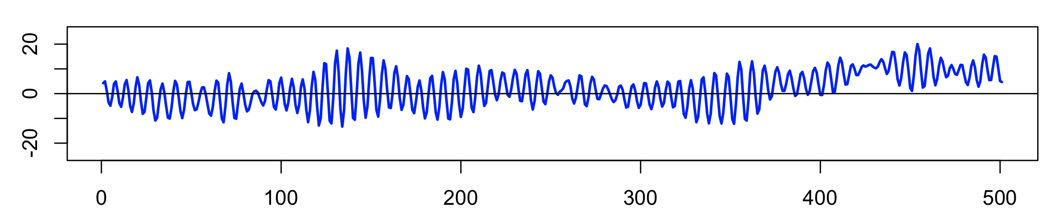
The MATRIX command above output the simulated time series to the file s1.txt: here is five seconds of the signal:

We also applied the PSD command to the newly generated signal S1, to use Welch method to estimate the spectrum from the data. Plotting the expected (gray line, same as above) against the estimated values for this one epoch, we see a good agreement: (note, there the lowest frequency estimated is 0.5 Hz, as the Welch method uses, by default, 4 second sliding windows; thus the x-axis is shifted relative to the plot above):

We can add the slope option to PSD to estimate the spectral slope using a simple linear regression on the log-log spectrum: i.e. the final PSD command were instead written:

PSD spectrum max=50 slope=30,45

then we can output the SLOPE as follows:

destrat out.db +PSD -r CH  | behead

We see the estimated value is close to the expected ( b = minus alpha ~ -2 ).

            ID   .                   
            CH   S1                  
            NE   1                   
    SPEC_SLOPE   -2.0451
  SPEC_SLOPE_N   61

In the above example we specified that the slope be estimated only over the region 30 to 45 Hz (as we and others have shown to be a robust choice, being relatively free from stronger oscillatoary activity and/or line noise (Kozhemiako et al, 2021).

If we had specified a broad range, that includes the (in this example, extremely strong) bump at 15 Hz, this naturally would have biased the slope estimate, which is now closer to 5 or 6.

PSD spectrum max=50 slope=10,45

            ID   .                   
            CH   S1                  
            NE   1                   
    SPEC_SLOPE   -5.6164   
  SPEC_SLOPE_N   141

See here for more details on the PSD and slope commands/options.

As a second example, here we base the simulation on a real power spectrum, estimated from N2 sleep, e.g. here from one individual from the NSRR CFS cohort (a random 10 minutes of N2 sleep):

luna cfs.lst 1 -o out.db -s ' MASK ifnot=N2 & RE
                              MASK random=20 & RE
                              PSD spectrum sig=C3 min=0 max=50 '

Note how we use the PSD options min and max along with spectrum to extract a broader range than the PSD command typically gives. We can extract the power spectrum to a file s.txt:

destrat out.db +PSD -r F CH > s.txt

To now simulate a time series with a similar power spectrum, we can use SIMUL and file: here, we simulate 6 minutes of signal (i.e. 180 one-second records) and read in the spectrum from s.txt:

luna . -o out.db --nr=180 --rs=1 -s ' SIMUL sr=400 file=s.txt sig=S1 verbose
                                      PSD spectrum max=200 '

By default, Luna assumes the PSD values are raw and not logged; if Luna detects a negative value in PSD it will assume they are 10log10(X) values (i.e. generated by PSD spectrum dB) and will convert them accordingly.

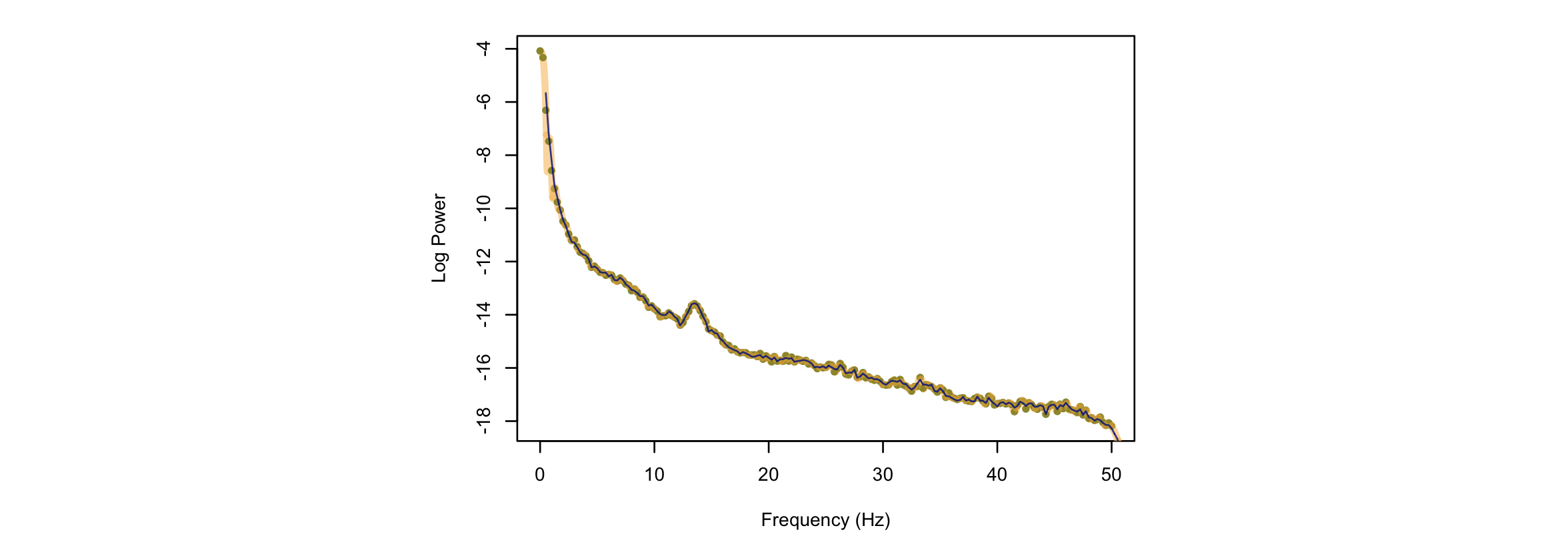
If we plot a) the original power spectra (with log(X) scaling), b) the interpolated expected spectra (orange, i.e. to match the given sample rate of 400 Hz), c) the estimated power spectra obtained via the Welch method to 180-seconds of randomly simulated data, as green, orange and navy points/lines respectively, we see they all line up more or less as expected:

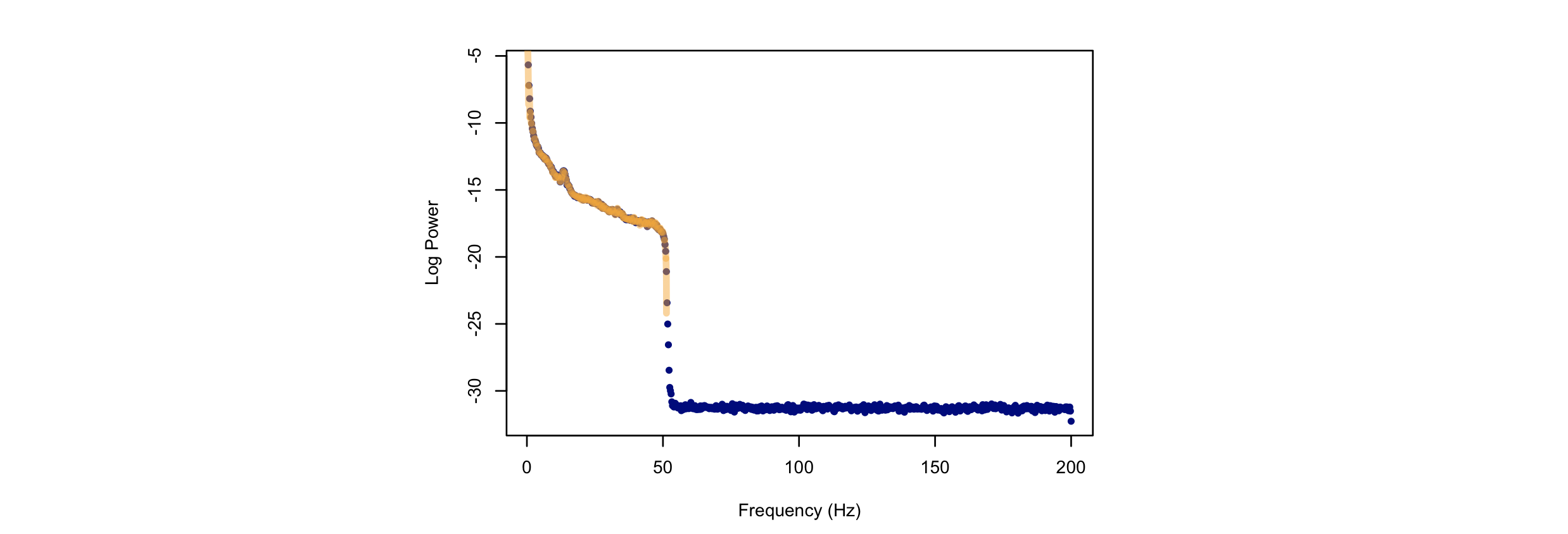
Note that we used a different sample rate here (400 Hz), which implies a different Nyquist frequency. The original spectrum was output up to 50 Hz. Implicitly, all unspecified frequencies are set to zero, when reading from a file: for a sample rate of 400 Hz for the generated signal, this implies values from 50 up to 200 Hz. Indeed, if we plot the full range of output from the previous SIMUL command, we'll see the spectrum extends up to 200 Hz, but with values of 0 for all frequencies above 50 Hz (which are therefore not defined on the log scale, and so are NA):

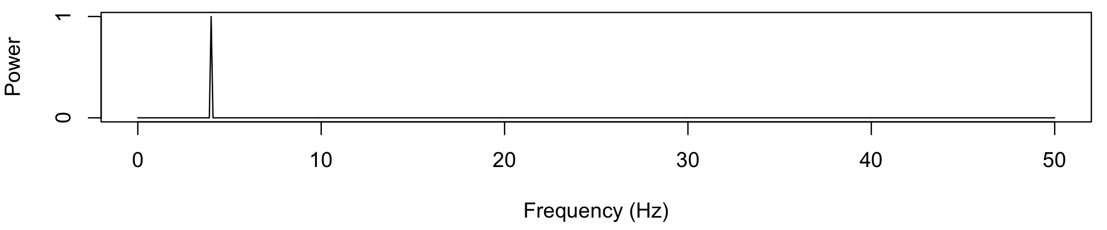
Finally, here we demonstrate the use of the pulses option, as well as adding different signals together. Below, we simulate 3 different 10-second segments. First, a constant 4 Hz sine wave:

luna . -o out.db --nr=10 --rs=1 \
       -s ' EPOCH len=10
            SIMUL sr=100 frq=4 psd=1 sig=S1
            FFT
            MATRIX minimal file=s1.txt '

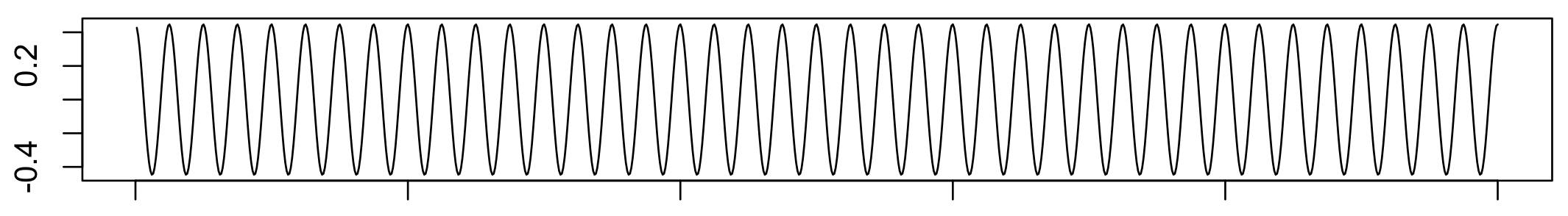
Note that we set the epoch length to 10 seconds (smaller than the default of 30 seconds), which ensures that subsequent commands operate correctly on a segment of data smaller than 30 seconds. We also use the FFT command to output the power spectrum associated with the new signal, which uses the basic DFT algorithm (rather than Welch or multi-taper approaches to spectral estimation). Plotting the contents of s1.txt (i.e. the raw time-domain signal output by MATRIX):

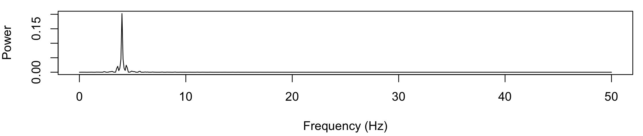
The second signal adds the pulses option to make the output consist of 3 segments (each of 1.5 second duration) within the overall 10-second window. As noted above, this is constrained to ensure that the segments do not overlap:

luna . -o out.db --nr=10 --rs=1
       -s ' EPOCH len=10
            SIMUL sr=100 frq=4 psd=1 sig=S1 pulses=3,1.5
            FFT
            MATRIX minimal file=s2.txt '

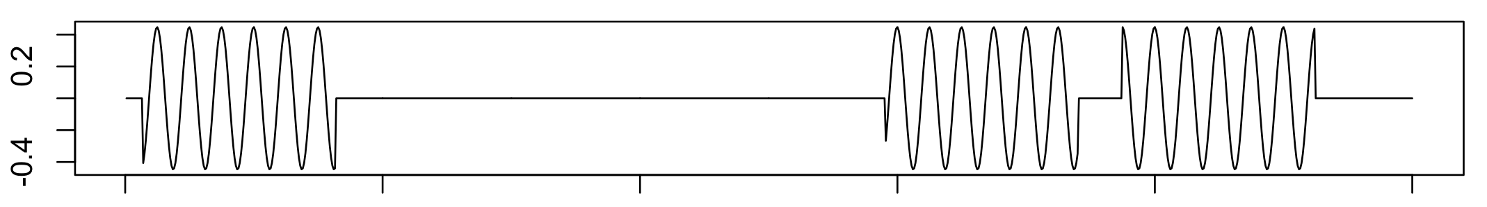
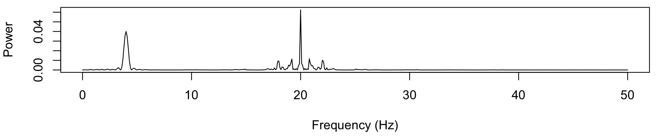
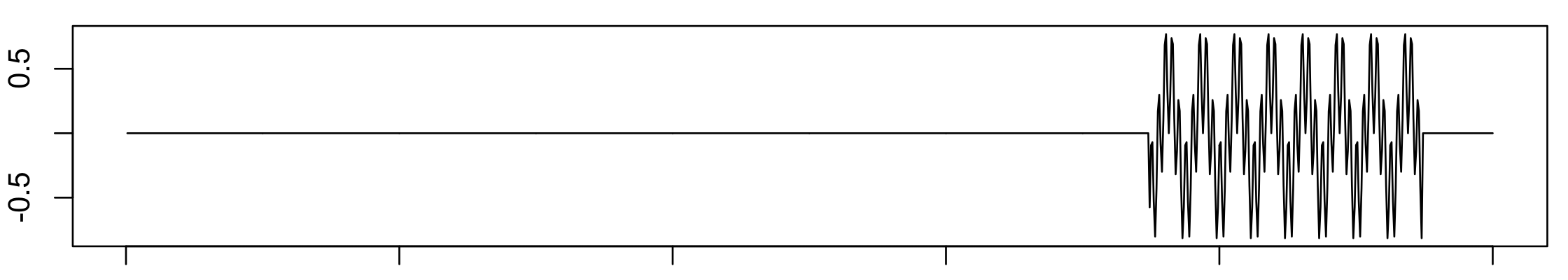
In this third example, we create two signals and add them together: a single 2-second segment of 4 Hz activity, and then superimpose 10 0.25-second segments of 20 Hz activity:

luna . -o out.db --nr=10 --rs=1 \
       -s ' EPOCH len=10
            SIMUL sr=100 frq=4  psd=1 sig=S1 pulses=1,2
            SIMUL sr=100 frq=20 psd=1 sig=S1 add pulses=10,0.25
            FFT
            MATRIX minimal file=s3.txt '

Now, for each of these three signals, we can look at power spectra obtained from the FFT command, extracting out output as:

destrat out.db +FFT -r F CH > o.1

The first shows the simple 4 Hz sine wave:

The second shows an attenuated peak at 4 Hz, with the discontinuities at the start/stop of segments introducing other spectral components:

Finally, we see a similar picture for the third signal, but with spectral components around both 4 and 20 Hz, again with the 'ripples' in the frequency domain resulting from the onsets/offsets of the pulses:

In this example, we've added two signals together, where the first was created from scratch. It is also possible to use add to modify an existing signal, if so desired.

Finally, also note that the frq and psd commands can accept multiple frequency/power pairs, but the pulses only acts on the composite signal generated:

luna . -o out.db --nr=10 --rs=1 \
       -s ' EPOCH len=10
            SIMUL sr=100 frq=4,20 psd=1,1 sig=S1 pulses=1,2
            FFT
            MATRIX minimal file=s3b.txt '

SIGGEN

Generate, or add-in, artificial test signals

This command is largely redundant (given SIMUL), but is decribed here for completeness.

This is a simple command to generate test signal data (on top of an existing EDF). Currently, it only generates sine wave signals, or pulses of a given duration.

Parameters

Parameter	Example	Description
`sig`	`sig=C3,C4`	Signals to be modified/created (existing or new)
`sr`	200	Set sample rate if not an existing channel
`add`		Add to an existing channel (versus overwrite it)
`sine`	`sine=10,20`	Generate a sine wave with specified frequency (10 Hz), amplitude (20 units) and optionally phase
`impulse`	`impulse=0.5,1,100`	Set impulse of amplitude `1` for 100 samples, starting at 0.5 way through the recording; multiple values are possible `impulse=T,A,D,T,A,D,...` , i.e. time/amplitude/duration

Output

No new output, this command just modifies the internal signal data.

Example

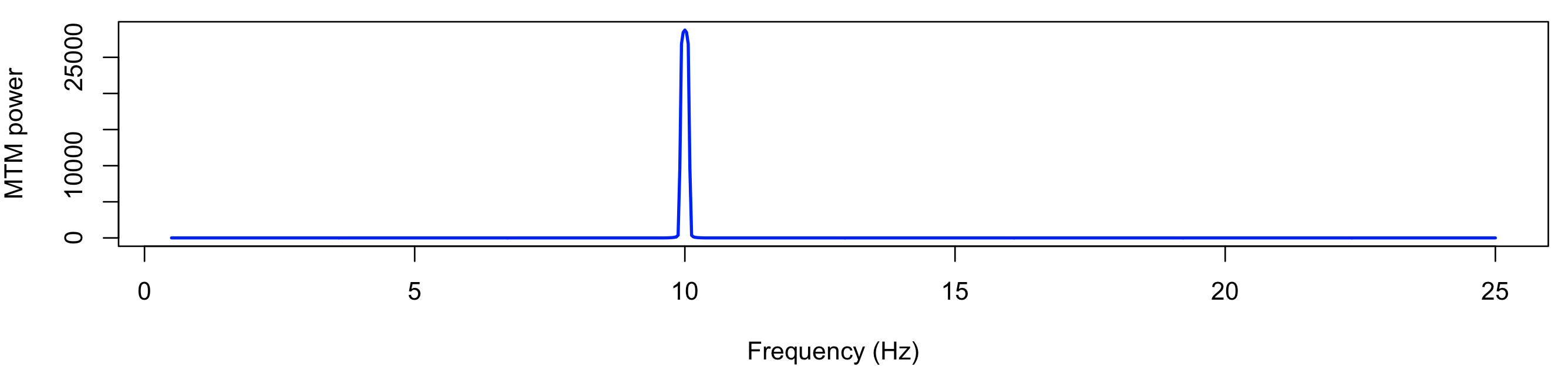
To generate a sine wave in the signal C3 (first clearing that signal):

luna s.lst -o out.db -s ' MASK ifnot=NREM2 & RE
                          SIGGEN sig=C3 clear sine=10,100 
                          MTM sig=C3 '

Plotting the output of MTM:

Also, see this vignette for an example of using SIGGEN to generate a toy dataset.