/R/epeat
In this section, we'll repeat the steps of the previous three tutorial pages, but using lunaR instead of lunaC. That is, these sections mirror the sections from the past three tutorials, and we'll try to accomplish the same goals but by different means..
For now, the easiest way to obtain lunaR is via one of the two Docker images, in which both Luna and the tutorial data are bundled with either classic R or RStudio. Here we'll use RStudio so that we can interactively view graphics created along the way. (Aside from being able to view graphics immediately, all other steps can be equally carried out via either route.)
As described in more detail on this page, once you've installed the free Docker Desktop client, you can download and initiate the container with a single command:
docker run -e PASSWORD=abc123 -p 8787:8787 remnrem/luna
Docker will look for an image called remnrem/luna and if it is not
found locally (i.e. it won't be on you first running this command), it
will automatically download it, during which time you'll see something
like this:
Unable to find image 'remnrem/luna:latest' locally
latest: Pulling from remnrem/luna
22dbe790f715: Extracting [============================>     ]  37.62MB/45.34MB
4bda69fb795b: Downloading [=============>                   ]   66.1MB/204.9MB
a9bef4c97d96: Downloading [============================>    ]  98.37MB/122.1MB
90ec09c6bb70: Download complete
b4333f4fff5d: Waiting
8affb09c10ec: Waiting
0d00367ae604: Waiting
94ec4d08d2c2: Waiting
954a0ad24247: Waiting
fa5834f7ad81: Waiting
The two other options on the command line above (i.e. -e and -p)
specified the new password you'll use when starting RStudio (for this
particular example, you can set it to anything) and mapped port 8787
from the container to your host machine. When the above command has
finished running, go to your browser and go to the following URL:
http://localhost:8787
If it asks you for a username and password, login with user-name
rstudio and the password you specified above
(i.e. abc123 in this example):
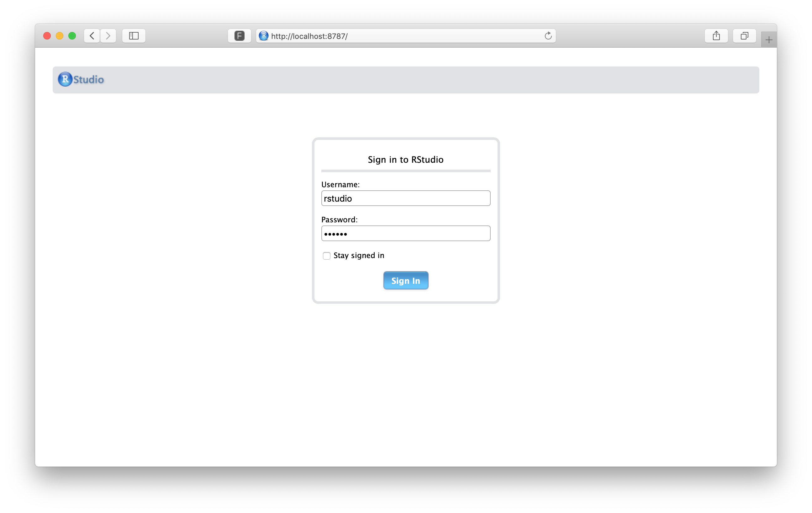
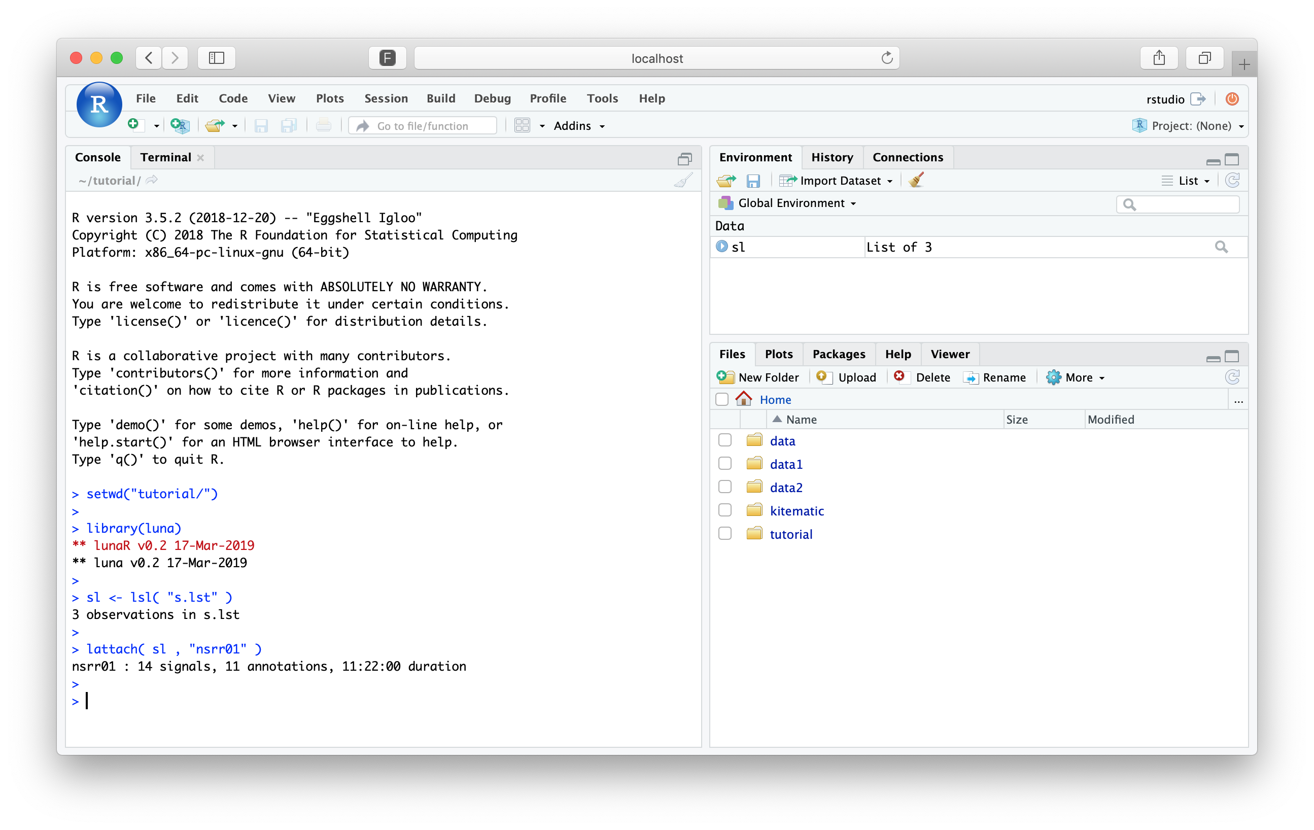
This will bring up the RStudio environment, which is running as a server within the Docker container, and which you access via port 8787 and your web browser. If you're not familiar with R or RStudio, there are lots of good tutorials available on-line if you search around.
Hint
For macOS and Linux users with the luna.docker bash script installed, all the above can be accomplished with:
luna.docker -rs abc123
Obtaining the data
The tutorial data are pre-installed in this image, under the
/tutorial folder. Let's start by making a copy of this folder (so new can potentially manipulate it)
to the home folder inside the container image. Go to the Terminal tab (next to the Console)
tab in RStudio to get a command line: first ensure you are in the home folder:
cd ~
/tutorial folder to the current location (.):
cp -r /tutorial .
setwd("~/tutorial/")
dir()
[1] "cmd" "edfs" "s.lst"
We'll also need to attach the lunaR library with the following command:
library(luna)
Displaying EDF files
Previous material
The corresponding section of the original tutorial covered:
- the
DESCto obtain basic information on EDFs, essentially just stepping through this command:
luna s.lst -s DESC > res.txt
To mirror the previous operations, we must first load a
sample-list with lunaR's
lsl() function:
sl <- lsl( "s.lst" )
This function returns the sample-list as an R list object, here
named sl. We can use lunaR's lattach()
function to start working with the first individual, nsrr01, by
passing by the sample-list and the ID (or the line number) of the
individual we want to attach:
lattach( sl , "nsrr01" )
Mirroring how lunaC processes a script (i.e. a set of Luna
commands either after the -s option or from a
command file), in lunaR we can
use the leval() (or
leval.project()) commands to process
Luna commands such as DESC. As for lunaC, the DESC command just
displays some information on the terminal, rather than sending output
to the formal output mechanism (i.e. a lunout database). The same is
true in lunaR:
leval( "DESC" )
EDF filename      : edfs/learn-nsrr01.edf
ID                : nsrr01
Clock time        : 21.58.17 - 09.20.16
Duration          : 11:22:00  40920 sec
# signals         : 14
Signals           : SaO2[1] PR[1] EEG_sec[125] ECG[250] EMG[125] EOG_L[50]
                    EOG_R[50] EEG[125] AIRFLOW[10] THOR_RES[10] ABDO_RES[10] POSITION[1]
                    LIGHT[1] OX_STAT[1]
To recap: here we've used a combination of lunaR commands to recapitulate the simple lunaC statement above:
lsl()to load a sample list calleds.lstlattach()to tell Luna which EDF we're interested inleval()to evaluate a Luna command, the same as the-soption in lunaC
Signal summary statistics
Previous context
The corresponding section of the original tutorial covered:
- running the
STATScommand for all three tutorial individuals - saving the output to a lunout database
- querying it with
destrat
One difference between lunaC and lunaR is that, with a few
exceptions, an attach EDF persists in-memory after a leval()
function has been performed. That is, the effects of any leval()
call that modifies the data (such as FILTER or SIGNALS or MASK)
will carry over for the next leval(), up until a new EDF is
lattach()-ed, or a lrefresh() command is issued to restore the EDF
to its original state. Therefore, unless you did something to make it
otherwise, the EDF for nsrr01 will still be in memory from the
previous analysis. We can confirm what the currently attached EDF is
(if any) with the lstat() command:
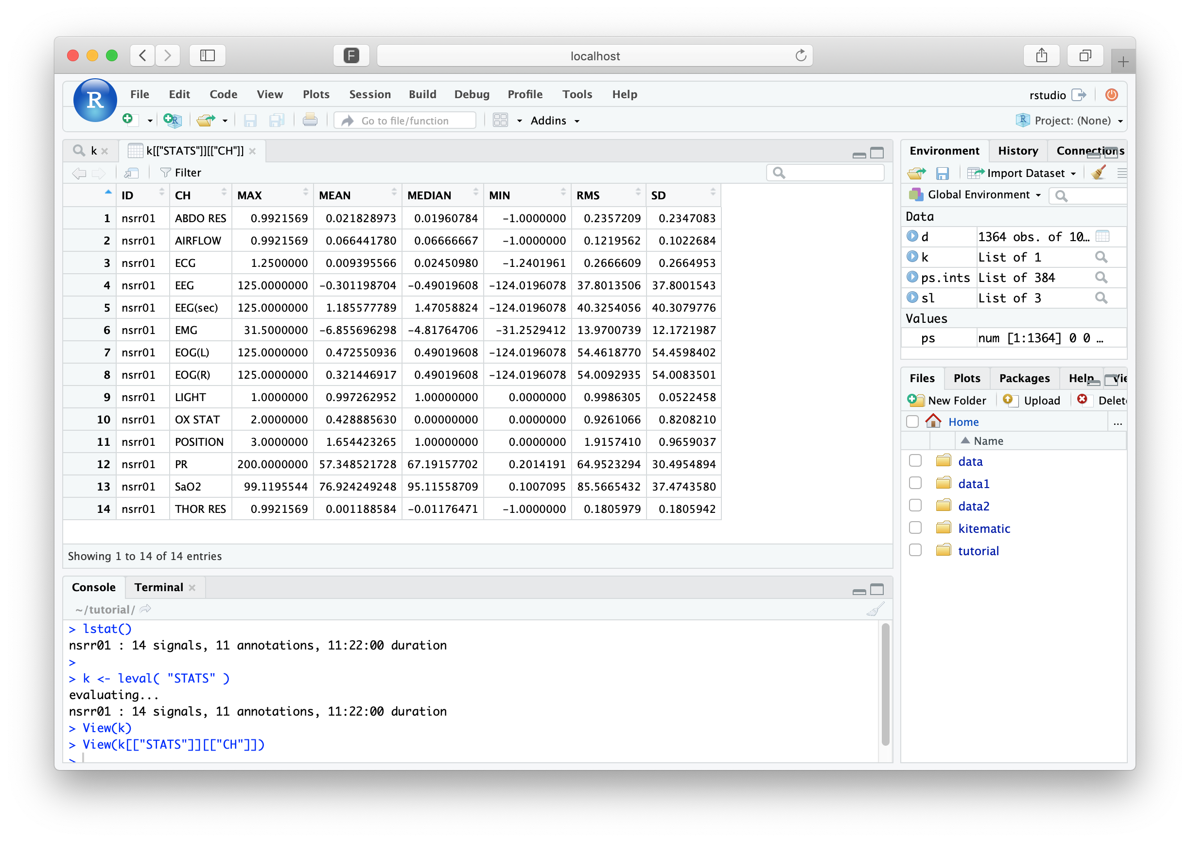
lstat()
nsrr01 : 14 signals, 11 annotations, 11:22:00 duration
To run the STATS command, we issue another leval():
k <- leval( "STATS" )
evaluating...
nsrr01 : 14 signals, 11 annotations, 11:22:00 duration
Unlike the DESC command,
STATS returns information to the formal
output mechanism: this is why we've assigned the return value of
leval() to be a new R object, called k.
Hint
leval() returns its output silently, in that you won't
see anything printed to the console if you do not assign the
output to another object. This doesn't mean the commands
weren't performed: masks, filters, etc, will still
modify the internal EDF.
The returned value k represents the same information that would have
been sent to the out.db database, if running this command in lunaC
from the command line. Similar to how destrat
summarizes a database, in lunaR the lx() command gives a simple
summary of a what leval() returns:
lx(k)
STATS : CH
That is, in this simple example, we have one command (STATS) and
one output table (defined by channel, CH). Using R's str()
function reveals more about the structure of k:
str(k)
List of 1
 $ STATS:List of 1
  ..$ CH:'data.frame':  14 obs. of  23 variables:
  .. ..$ ID  : chr [1:14] "nsrr01" "nsrr01" "nsrr01" "nsrr01" ...
  .. ..$ CH  : chr [1:14] "ABDO_RES" "AIRFLOW" "ECG" "EEG" ...
  .. ..$ MAX : num [1:14] 0.992 0.992 1.25 125 125 ...
  .. ..$ MEAN: num [1:14] 0.0218 0.0664 0.0094 -0.3012 1.1856 ...
  .. ..$ MIN : num [1:14] -1 -1 -1.24 -124.02 -124.02 ...
  .. ..$ P01 : num [1:14] -0.71 -0.2 -1.24 -124.02 -124.02 ...
  .. ..$ P02 : num [1:14] -0.506 -0.129 -0.858 -124.02 -124.02 ...
  .. ..$ P05 : num [1:14] -0.3176 -0.0667 -0.1912 -70.098 -78.9216 ...
  .. ..$ P10 : num [1:14] -0.2 -0.0275 -0.0833 -24.0196 -20.098 ...
  .. ..$ P20 : num [1:14] -0.0902 0.0118 -0.0343 -9.3137 -7.3529 ...
  .. ..$ P30 : num [1:14] -0.0196 0.0353 -0.0049 -5.3922 -3.4314 ...
  .. ..$ P40 : num [1:14] 0.00392 0.05098 0.01471 -2.45098 -0.4902 ...
  .. ..$ P50 : num [1:14] 0.0196 0.0667 0.0245 -0.4902 1.4706 ...
  .. ..$ P60 : num [1:14] 0.0275 0.0745 0.0245 2.451 3.4314 ...
  .. ..$ P70 : num [1:14] 0.051 0.0902 0.0343 4.4118 6.3725 ...
  .. ..$ P80 : num [1:14] 0.098 0.1137 0.0343 8.3333 10.2941 ...
  .. ..$ P90 : num [1:14] 0.2627 0.1608 0.0833 23.0392 22.0588 ...
  .. ..$ P95 : num [1:14] 0.435 0.208 0.211 72.059 78.922 ...
  .. ..$ P98 : num [1:14] 0.663 0.278 0.828 125 125 ...
  .. ..$ P99 : num [1:14] 0.875 0.349 1.25 125 125 ...
  .. ..$ RMS : num [1:14] 0.236 0.122 0.267 37.801 40.325 ...
  .. ..$ SD  : num [1:14] 0.235 0.102 0.266 37.8 40.308 ...
  .. ..$ SKEW: num [1:14] 0.3348 0.1384 -0.1152 0.0862 -0.0688 ...
To see the entire list (that really only contains one data frame), just type k:
k
$STATS
$STATS$CH
       ID       CH      MAX      MEAN    MEDIAN      MIN     RMS      SD
1  nsrr01 ABDO RES   0.9921  0.021828  0.01960   -1.0000  0.2357  0.2347
2  nsrr01  AIRFLOW   0.9921  0.066441  0.06666   -1.0000  0.1219  0.1022
3  nsrr01      ECG   1.2500  0.009395  0.02450   -1.2401  0.2666  0.2664
4  nsrr01      EEG 125.0000 -0.301198 -0.49019 -124.0196 37.8013 37.8001
5  nsrr01 EEG(sec) 125.0000  1.185577  1.47058 -124.0196 40.3254 40.3079
6  nsrr01      EMG  31.5000 -6.855696 -4.81764  -31.2529 13.9700 12.1721
7  nsrr01   EOG(L) 125.0000  0.472550  0.49019 -124.0196 54.4618 54.4598
8  nsrr01   EOG(R) 125.0000  0.321446  0.49019 -124.0196 54.0092 54.0083
9  nsrr01    LIGHT   1.0000  0.997262  1.00000    0.0000  0.9986  0.0522
10 nsrr01  OX STAT   2.0000  0.428885  0.00000    0.0000  0.9261  0.8208
11 nsrr01 POSITION   3.0000  1.654423  1.00000    0.0000  1.9157  0.9659
12 nsrr01       PR 200.0000 57.348521 67.19157    0.2014 64.9523 30.4954
13 nsrr01     SaO2  99.1195 76.924249 95.11558    0.1007 85.5665 37.4743
14 nsrr01 THOR RES   0.9921  0.001188 -0.01176   -1.0000  0.1805  0.1805
That is, we have statistics for 14 channels from one tutorial
individual, nsrr01. However, the original lunaC command
calculated and compiled results for all three studies in the project.
Obviously, we could write a simple loop to achieve this in R,
repeatedly calling lattach() and leval() and compiling results.
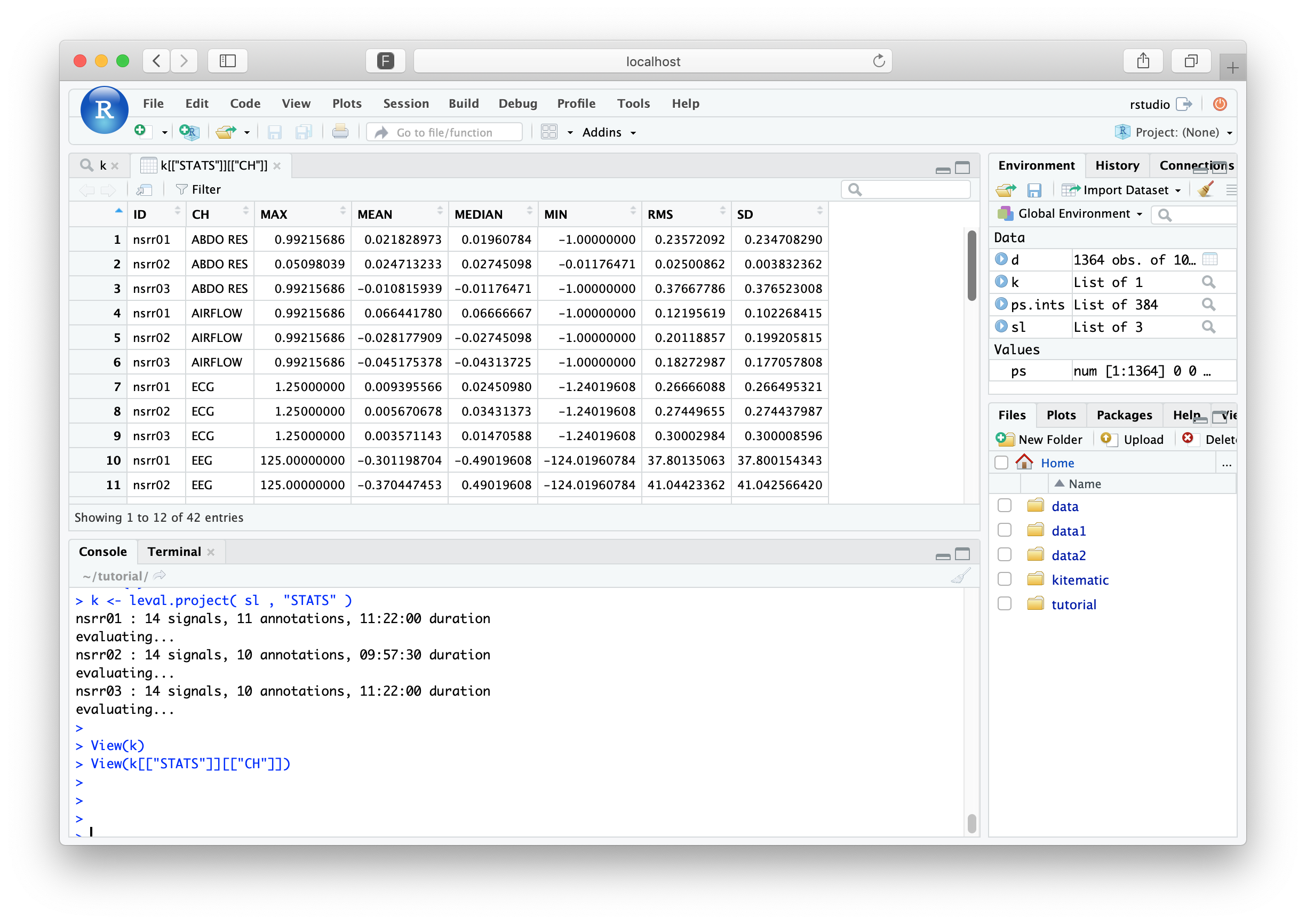
Alternatively, an easier way to do this is the leval.project()
function instead, which performs pretty much the same series of
operations as lunaC does. That is, the luna_C statement:
luna s.lst -o out.db -s STATS
k <- leval.project( sl , "STATS" )
where sl is the the file s.lst (attached with lsl()) and k is
the equivalent of out.db.
The returned value, k now contains results for all three
individuals. Although the overall structure is the same as before,
each data-frame now has additional rows for the additional individuals
(with the ID column indicating who's who). In RStudio, you can
explore the results by clicking on k in the Environment tab, or by
typing
View(k)
To mirror the previous tutorial section, we need now to extract the
"signal means for the ECG, EMG and SaO2". Here we can use the
lx() function with an additional parameter (the command
name), which will, in this case (as there is only a single table
associated with this command's output) will return a data-frame with
the output:
d <- lx( k , "STATS" )
MEAN) along with
ID and CH columns:
names(d)
 [1] "ID"   "CH"   "KURT" "MAX"  "MEAN" "MIN"  "P01"  "P02"  "P05"  "P10"  "P20"
[12] "P30"  "P40"  "P50"  "P60"  "P70"  "P80"  "P90"  "P95"  "P98"  "P99"  "RMS"
[23] "SD"   "SKEW"
d[ d$CH %in% c("ECG","EMG","SaO2") , c("ID","CH","MEAN") ]
       ID   CH         MEAN
7  nsrr01  ECG  0.009395566
8  nsrr02  ECG  0.005670678
9  nsrr03  ECG  0.003571143
16 nsrr01  EMG -6.855696298
17 nsrr02  EMG -0.609767419
18 nsrr03  EMG  3.013591554
37 nsrr01 SaO2 76.926126702
38 nsrr02 SaO2 77.874804354
39 nsrr03 SaO2 65.084439075
Working with annotations
Previous material
The corresponding section of the original tutorial covered:
- looking at the contents of an NSRR XML annotation file
- counting the number of apnea events per individual, either for the whole night, or specific to REM sleep
When we attach an EDF with lattach(), if the sample list specified
any annotation files, they too are automatically loaded. For example,
considering nsrr01, when we attach that dataset, we see there are 11
annotation classes are also attached (i.e. from the XML file specified
in s.lst):
lattach( sl , 1 )
nsrr01 : 14 signals, 11 annotations, 11:22:00 duration
To see what those annotations classes are, we can use the lannots() command:
lannots()
 [1] "Arousal"           "Hypopnea"          "N1"
 [4] "N2"                "N3"                "Obstructive_Apnea"
 [7] "R"                 "SpO2_artifact"     "SpO2_desaturation"
lannots() with a single annotation class name as a parameter, we'll get a list of
the intervals (in seconds elapsed since the start of the EDF):
lannots( "Obstructive_Apnea" )
[[1]]
[1] 2300.7 2310.7

[[2]]
[1] 2329.6 2343.1

[[3]]
[1] 4933.6 4953.2

[[4]]
[1] 5064.9 5095.1

[[5]]
[1] 5248.1 5265.5

... (cont'd) ...
That is, the first apnea event was from 2300.7 to 2310.7 seconds (10 seconds); the second was from 2329.6 to 2343.1 seconds (13.5 seconds), etc.
Luna's masks work in terms of
epochs, which are fixed intervals spanning the
recording (by default, typically 30 seconds). We can see how epochs
and annotations line up with the letable()
(epoch-table) command. First, we need to specify epochs for this
record:
lepoch()
nsrr01 : 14 signals, 11 annotations, 11:22:00 duration, 1364 unmasked 30-sec epochs, and 0 masked
The output from lstat() now additionally includes information about
the number of epochs, and whether or not they are currently masked.
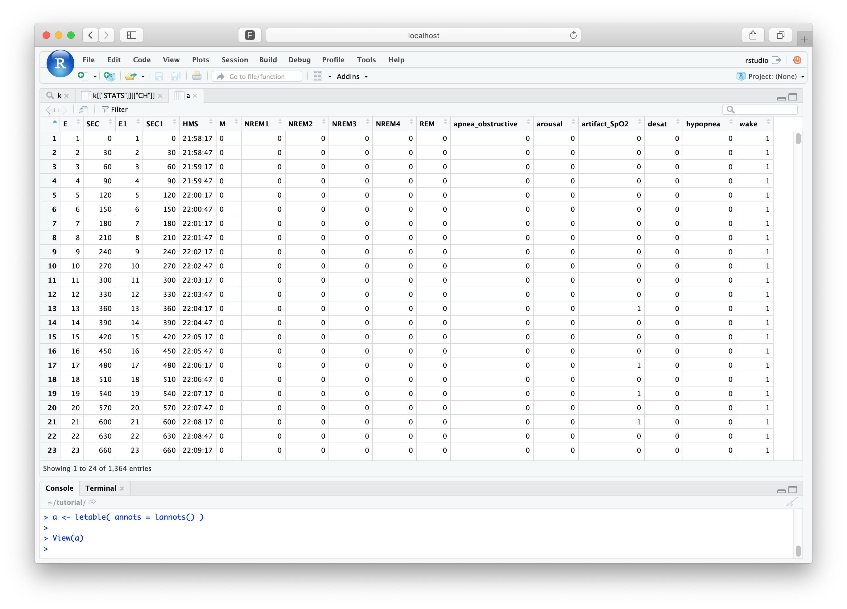
To explore the epoch structure in more detail, along-side annotation
information, we can use letable() to tabulate all epochs (when they
occur, whether they are masked or not, and, if the EDF has been
restructured, how that epoch maps to the original EDF):
a <- letable( annots = lannots() )
Quickly summarizing sleep stages
One other convenience
function is lstages(), which is just a wrapper
around the evaluation of the Luna
STAGES command and returns a
vector of sleep stage labels (e..g NREM1, NREM2, etc) per
epoch. Stage labels must exist as annotations (i.e. this command
does not automatically infer sleep stage on-the-fly from the raw
signal data_).
ss <- lstages()
table( ss )
 N1  N2  N3   R   W
109 523  17 238 477
All NSRR data have annotations formatted in such a way as to work with these commands, although it is easy to modify this to work with other formats.
Moving on the question of the original tutorial section: how can we
count the number of apneas per individual? As previously, we'll use the
ANNOTS command, combined with leval.project() to
apply this to each individual:
k <- leval.project( sl, "ANNOTS" )
As described on the ANNOTS command page,
counts of annotation instances for each annotation class are in the table stratified by ANNOT:
lx(k)
ANNOTS : ANNOT ANNOT_INST ANNOT_INST_T1_T2
We can simply extract this with lx( k , "ANNOTS" , "ANNOT" ), or
alternatively, just write it directly:
d <- k$ANNOTS$ANNOT
If we restrict to rows where the annotation class name is Obstructive_Apnea, we'll see that COUNTs
for each individual.
d[ d$ANNOT == "Obstructive_Apnea" , ]
       ID             ANNOT COUNT    DUR
14 nsrr01 Obstructive_Apnea    37  824.5
15 nsrr02 Obstructive_Apnea     5   67.7
16 nsrr03 Obstructive_Apnea   163 3795.6
Reassuringly, these match what was obtained in the previous tutorial
section. To consider only events during REM, we can re-run but including a
MASK statement:
k <- leval.project( sl , "MASK ifnot=R & ANNOTS" )
Repeating the above steps to extract the output:
d <- k$ANNOTS$ANNOT
d[ d$ANNOT == "Obstructive_Apnea" , ]
      ID             ANNOT COUNT   DUR
7 nsrr01 Obstructive_Apnea    27 668.4
8 nsrr02 Obstructive_Apnea     3  43.4
Again, these results match what we observed with lunaC.
Putting it together
Previous material
The corresponding section of the original tutorial covered:
Up to now, we've directly entered Luna commands as text on the R
command line. We can also read command
files in the same way that lunaC
does, which is recommended for all non-trivial applications. The lunaR function lcmd()
will read and parse a Luna-format command file, and return a vector where each instruction in one element:
lcmd( "cmd/first.txt" )
[1] "EPOCH len=30"           "TAG tag=STAGE/${stage}" "MASK ifnot=${stage}"
[4] "RESTRUCTURE"            "STATS sig=EEG"
That is, lcmd() strips away comments (%) and blank lines, etc. As
well as using & to concatenate Luna commands, leval() and
leval.project() functions accept vectors of commands, so we can pass
the output of lcmd() to leval(), etc. However, you'll note from
looking at the commands above, we have one issue we need to first
resolve, namely the use of variables in
the command file. When using lunaC, we'd specify the value of
${stage} on the command line, as well as passing special variables such as
sig to define the signal list. For example,
luna s.lst stage=N1 sig=EEG -o out.db < cmd/first.txt
In lunaR, we can set Luna environment variables with the
lset() function:
lset( "stage","N1" )
setting [stage] to [N1]
We can query if a value exists, with lvar():
lvar("stage")
[1] "N1"
We can use a similar approach with sig, to specify which signal(s)
this analysis is restricted to:
lset( "sig" , "EEG" )
However, as sig is a special variable, it is treated a little differently:
-
because it is not a user-defined variable,
lvar("sig")will not show anything; the same is true when setting other special variables such asalias -
repeated calls setting to
sig(oralias) variables do not overwrite the earlier values; rather, they append to that list
Setting special variables in lunaR
In other words, after the commands:
lset( "sig" , "EEG1,EEG2" )
lset( "sig" , "EEG3" )
the signal-list will comprise all three signals, not just EEG3.
To clear the signal-list, use this special form:
lset( "sig" , "." )
lreset()
Having specified the value of ${stage} as well as the signal-list
(i.e. to restrict analysis to just the EEG channel), we can run
leval.project(), using lcmd() to read in and parse the command
script we used previously with lunaC:
k <- leval.project( sl , lcmd( "cmd/first.txt" ) )
k) with lx(), as before:
lx(k)
EPOCH : BL STAGE
MASK : EMASK_STAGE
RESTRUCTURE : STAGE
STATS : CH_STAGE
Note that each table also has STAGE as an additional factor, due to
the use of the TAG command. That is, these results
are currently just for NREM1 sleep:
lx( k , "STATS" )
      ID  CH STAGE      KURT       MAX         MEAN        MIN       P01       P02
1 nsrr01 EEG    N1  1.770623  59.31373 -0.295451220  -81.86275 -18.13725 -16.17647
2 nsrr02 EEG    N1  1.976144  49.50980  0.007177659  -72.05882 -28.92157 -23.03922
3 nsrr03 EEG    N1 37.534412 125.00000  0.198371041 -124.01961 -25.98039 -20.09804
        P05        P10       P20       P30       P40        P50      P60      P70      P80
1 -12.25490  -9.313725 -6.372549 -3.431373 -1.470588 -0.4901961 1.470588 3.431373 5.392157
2 -17.15686 -12.254902 -7.352941 -4.411765 -1.470588  0.4901961 2.450980 5.392157 8.333333
3 -14.21569 -10.294118 -6.372549 -3.431373 -1.470588  0.4901961 2.450980 4.411765 7.352941
        P90      P95      P98      P99       RMS        SD        SKEW
1  8.333333 11.27451 15.19608 18.13725  7.354944  7.349016  0.01513765
2 12.254902 16.17647 20.09804 24.01961 10.361542 10.361666 -0.48778254
3 11.274510 14.21569 20.09804 26.96078 12.302106 12.300538 -0.46132928
To obtain the values for other sleep stages, we can just repeat the above procedures. To facilitate this, and to make the output easier to collate, we'll do the following. First, we'll define the stages we want to iterate over:
stgs <- c( "N1", "N2", "N3" , "R" )
k <- list()
We then can use a for loop in R to iterate over each stage, setting
the appropriate ${stage} value, and then running the script:
for (s in stgs) {

 lset( "stage", s )

 k[[ s ]] <- leval.project( sl , lcmd( "cmd/first.txt" ) )

}
When this runs, you'll see a warning message displayed to the console for the last individual:
** skipping STATS as there are no unmasked records
This is fine and as expected: as we previously saw, this is because
nsrr03 doesn't have any REM epochs.
Hint
If you see other errors in lunaR, it
may often be that you forgot to lset()/lreset() any
variables, forgot to lattach() an individual, or need to
lrefresh() the attached EDF when running a new command, i.e. if there are
no unmasked records left for that EDF.
Note that rather than saving the output of leval.project() directly
to k, we are writing it to a sub-item of the existing list, using
sleep stage s as index an index. (A technical point, but R uses
double brackets [[ often when working with lists, to indicate any
single element itself, rather than [, which indicates a list of
the selected elements,
e.g. see here).
Persistence of EDFs in leval() and leval.project()
When using leval.project(), lunaR behaviors much more like lunaC in terms of the persistence of in-memory
EDFs. That is, each EDF in the sample list is attached and then dropped before moving to the next EDF in the list. So,
unlike leval(), which does not detach the EDF, this means that after running the above, there will not be any currently attached EDF:
lstat()
Error in lstat() : no EDF attached
More importantly, it means that when running leval.project()
inside a loop as above, any modifications made (e.g. from masks,
filters, dropping or adding signals, etc), will not be reflected
when re-running the loop. So, leval.project() is really like
running a single lunaC statement. In contrast, leval() works
more like the individual components that occur within one
lunaC run for one individual.
Having run the above code successfully, we'll now have a slightly
different format for k. Namely, it is a list with 4 elements,
correspond to the four sleep stages. Each element is identical to the
output that would have come from a single run of leval.project()
(obviously... that is how we assigned it above).
Therefore, lx() will work slightly differently, due to the structure of the output. By itself,
rather than returning each command as a row, along with a list of tables from that command, lx()
will now return each higher level group (i.e. s or sleep stage in this case), along with a list of the commands
performed:
lx(k)
N1 : EPOCH MASK RESTRUCTURE STATS
N2 : EPOCH MASK RESTRUCTURE STATS
N3 : EPOCH MASK RESTRUCTURE STATS
R : EPOCH MASK RESTRUCTURE STATS
We cannot use lx() to extract a particular table from a particular
command however. The alternative lx2() can be used in this
scenario, i.e. if and only if you've consciously structured the output in
the way we have above. So, instead if lx( k , "STATS" ), we'd run
lx2( k , "STATS" )
         ID  CH STAGE      KURT       MAX         MEAN        MIN       P01
N1.1 nsrr01 EEG    N1  1.770623  59.31373 -0.295451220  -81.86275 -18.13725
N1.2 nsrr02 EEG    N1  1.976144  49.50980  0.007177659  -72.05882 -28.92157
N1.3 nsrr03 EEG    N1 37.534412 125.00000  0.198371041 -124.01961 -25.98039
N2.1 nsrr01 EEG    N2  2.935892 125.00000 -0.313127132 -124.01961 -27.94118
N2.2 nsrr02 EEG    N2  6.550833 125.00000 -0.134945206 -124.01961 -40.68627
N2.3 nsrr03 EEG    N2 20.749735 125.00000  0.126607059 -124.01961 -37.74510
N3.1 nsrr01 EEG    N3  7.165718 121.07843 -0.454932718 -112.25490 -37.74510
N3.2 nsrr02 EEG    N3  1.547826 125.00000 -0.130731673 -124.01961 -51.47059
N3.3 nsrr03 EEG    N3  2.156775 125.00000  0.171914099 -124.01961 -47.54902
R.1  nsrr01 EEG     R  2.869020  85.78431 -0.371502169  -82.84314 -19.11765
R.2  nsrr02 EEG     R 22.273566 125.00000 -0.384220044 -124.01961 -44.60784
...
Because we used TAG in the script, we have a variable named STAGE
that corresponds to this higher-level structure, making it easy to
keep track of results.
So, to extract the same information as previously (namely, signal RMS for the EEG channel for all three individuals, stratified by sleep stage), we could run the following:
d <- lx2( k , "STATS")
d[ , c("ID","STAGE","RMS")]
         ID STAGE       RMS
N1.1 nsrr01    N1  7.354944
N1.2 nsrr02    N1 10.361542
N1.3 nsrr03    N1 12.302106
N2.1 nsrr01    N2 10.646079
N2.2 nsrr02    N2 14.742420
N2.3 nsrr03    N2 14.496728
N3.1 nsrr01    N3 13.014505
N3.2 nsrr02    N3 20.054659
N3.3 nsrr03    N3 18.980088
R.1  nsrr01     R  7.563595
R.2  nsrr02     R 14.146456
To get a nice tabulation, we could do the following: (although there are more efficient ways to do this, if needed):
with( d , tapply( RMS , list( ID , STAGE ) , mean ) )
              N1       N2       N3         R
nsrr01  7.354944 10.64608 13.01451  7.563595
nsrr02 10.361542 14.74242 20.05466 14.146456
nsrr03 12.302106 14.49673 18.98009        NA
Something strange about the medians?
You may have noted
that in the tables above, the MEDIAN values of the EEG were all
very similar numbers: either 0.49019 or -0.49019. Did we do
something wrong? In this case, no we didn't, it is simply a property of the resolution of the data after
analog to digital conversion. To use lunaR to check this out, let's attach one individual:
lattach( sl , 1 )
To pull an entire signal we can use ldata() but we need to
specify the interval in terms of epochs, so we must first epoch
the data (here, saving the number of epochs in ne):
ne <- lepoch()
We can then request the entire (1:ne) EEG signal (note, we
only keep the signal rather than the whole data frame returned by
ldata(): we'll add more efficient ways to extract only signals in
the future):
x <- ldata( 1:ne , "EEG" )$EEG
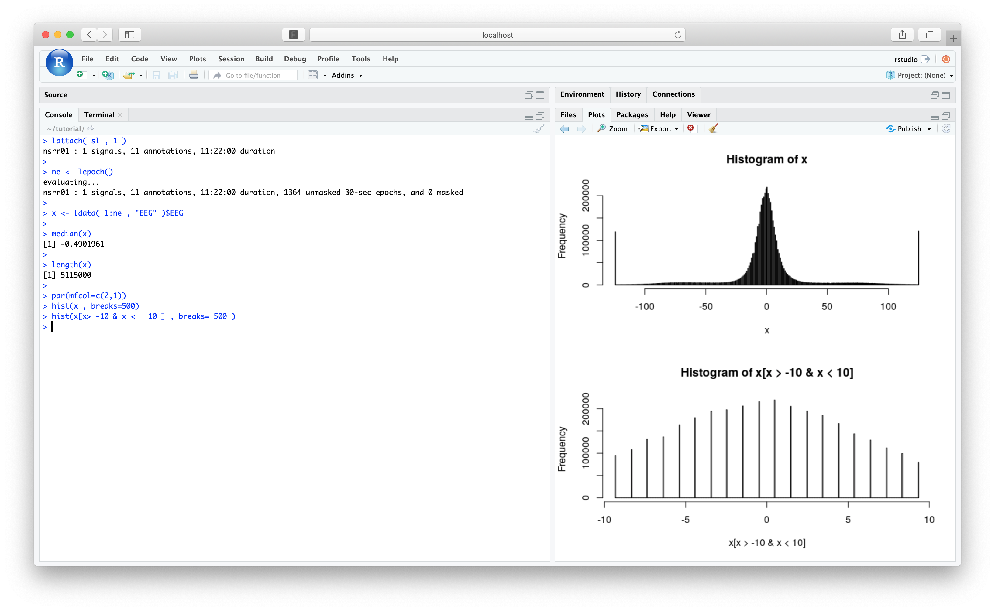
Let's check things are as expected: length(x) gives 5115000;
given we have 1364 30-second epochs and a sampling rate of 125 Hz,
this is good, as 1364 * 30 * 125 = 5115000. Now, to check the median:
median(x)
-0.4901961
We're seeing the same number as above in the stage-stratified analyses. Looking at the distribution of the samples, we see this simply reflects the resolution of the digital signal:
par(mfcol=c(2,1))
hist(x , breaks=500)
hist(x[x> -10 & x < 10 ] , breaks= 500 )
Using destrat
Previous material
The corresponding section of the original tutorial covered:
- how to use the
destrattool to work with the lunout databases generated by lunaC's-ooption
In lunaR we do not generate lunout databases;
rather, any commands executed return their results directly as R list
objects. (If you want to save any of these, you can simply use R's
standard save() function, or similar.) However, it is in fact
possible to read lunout databases generated by lunaC into lunaR,
with the ldb() function.
As a quick example, within RStudio, switch to the "Terminal" tab (instead of "Console"). This gives a prompt in a bash (Bourne Again Shell) where you can access the virtual Linux machine running RStudio:
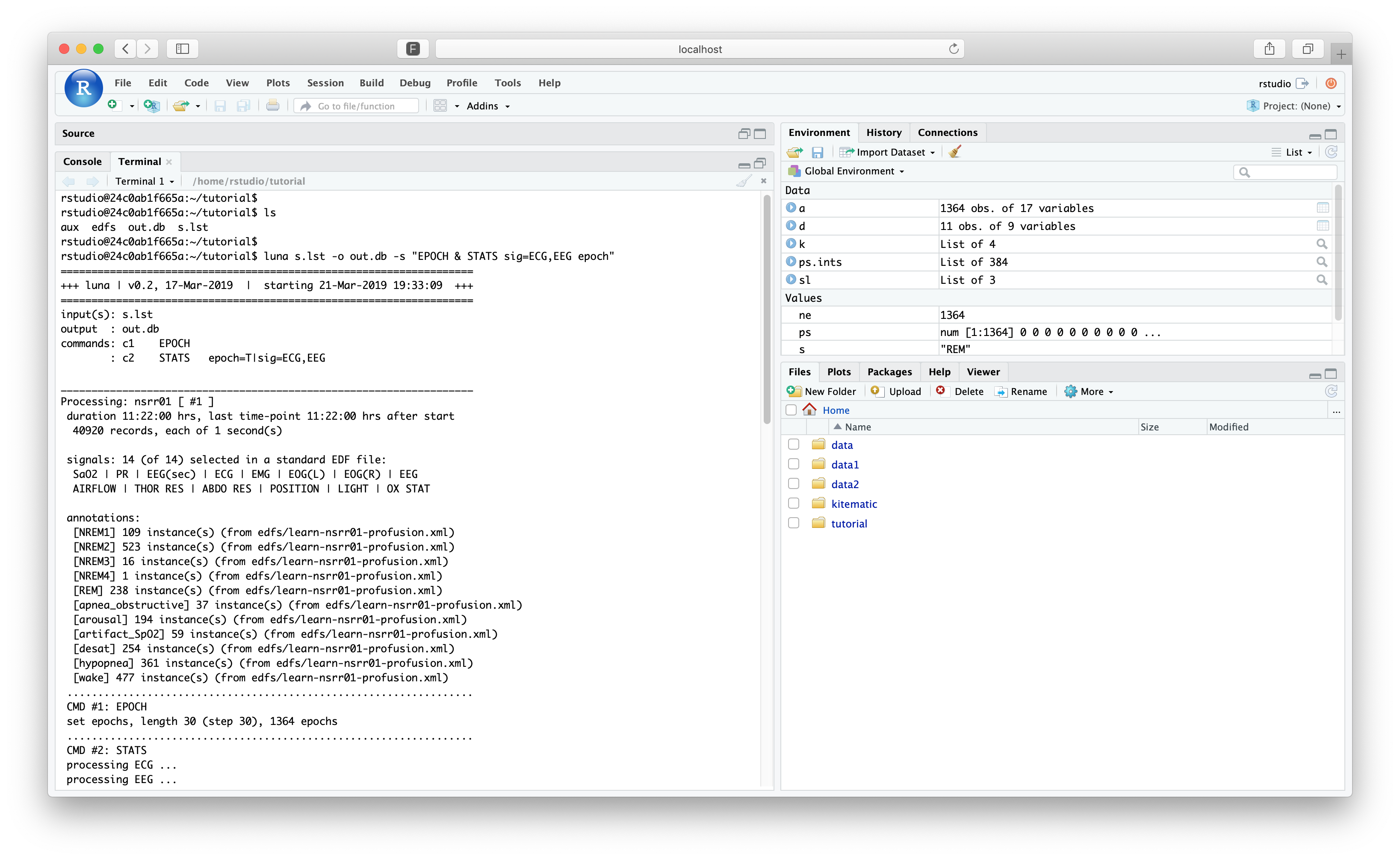
This should be in the same tutorial/ folder (if you are not, run cd
tutorial). Typing ls should show the s.lst file and the two
folders, edfs and cmd. Now run a command that generates an out.db file: e.g.
luna s.lst -o out.db -s "EPOCH & STATS sig=ECG,EEG epoch"
destrat out.db
--------------------------------------------------------------------------------
out.db: 2 command(s), 3 individual(s), 15 variable(s), 47157 values
--------------------------------------------------------------------------------
  command #1:   c1      Thu Mar 21 19:33:09 2019        EPOCH
  command #2:   c2      Thu Mar 21 19:33:09 2019        STATS
--------------------------------------------------------------------------------
distinct strata group(s):
  commands      : factors           : levels        : variables
----------------:-------------------:---------------:---------------------------
  [EPOCH]       : .                 : 1 level(s)    : DUR INC NE
                :                   :               :
  [EPOCH]       : CH                : 1 level(s)    : DUR INC NE
                :                   :               :
  [STATS]       : CH                : 2 level(s)    : MAX MEAN MEDIAN MEDIAN.MEAN MEDIAN.MEDIAN
                :                   :               : MEDIAN.RMS MEDIAN.SD MIN NE NE1
                :                   :               : RMS SD
                :                   :               :
  [STATS]       : E CH              : (...)         : MAX MEAN MEDIAN MIN RMS SD
                :                   :               :
----------------:-------------------:---------------:---------------------------
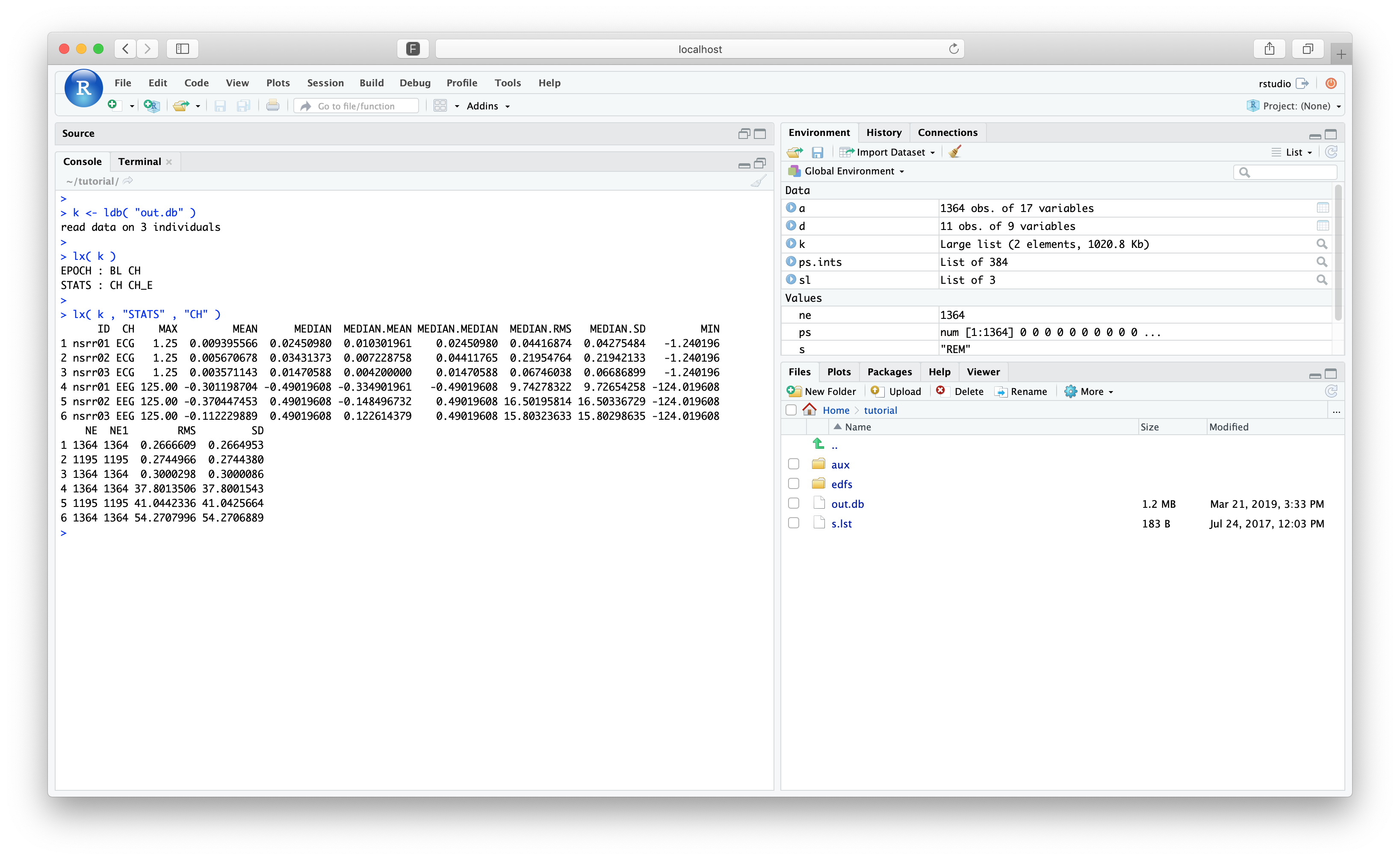
Switching back to the RStudio Console (i.e. back to the R prompt), you can read in that same output database
k <- ldb( "out.db" )
Note
Not all return objects have to be named k, I'm just a creature of habit...
Using lx(), we should see the same structure and information:
Parameter files
Previous material
The corresponding section of the original tutorial covered:
- using a parameter file to specify variables
- executing the command file
cmd/second.txtwith thecmd/vars.txtparameter file
You can use the lset() function to read in variable assignments from a parameter file.
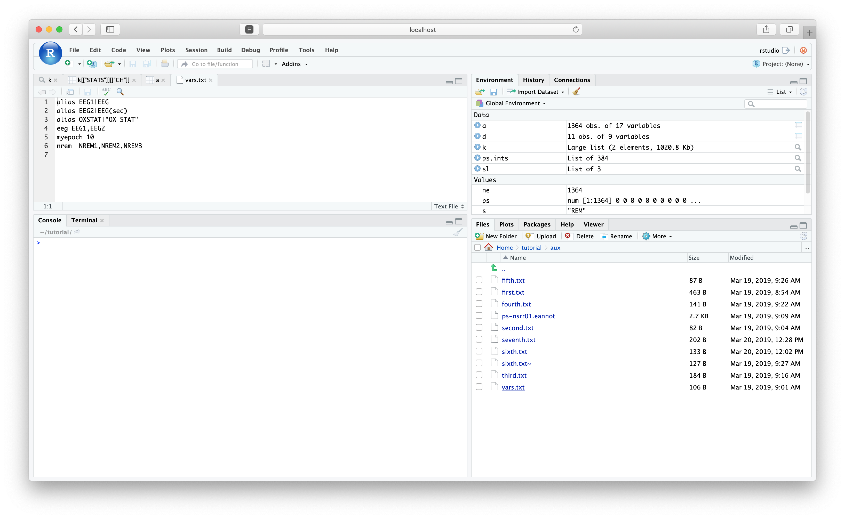
We previously used the file cmd/vars.txt, which we can view within RStudio by navigating to the
tutorial folder and clicking on that file:
The previous section ran the command file cmd/second.txt for
nsrr01, which basically just wrote some stats for the two EEG
channels. We'll start by attaching this EDF:
lattach( sl , "nsrr01" )
nsrr01 : 1 signals, 11 annotations, 11:22:00 duration
But wait! Isn't there a problem? This reads that only a single
signal is present, whereas there are 14 in that EDF. This isn't an
error: rather, it reflects a previously set Luna environment
variable, i.e. namely sig, the signal-list, from section
above. Within the same session, lunaR will remember these settings
(i.e. it is as if we're running every command with sig=EEG
included). When starting a new analysis, it is therefore a good idea
to first reset these variables, i.e. to start afresh.
lreset()
lattach( sl , "nsrr01" )
nsrr01 : 14 signals, 11 annotations, 11:22:00 duration
lchs():
lchs()
 [1] "SaO2"     "PR"       "EEG_sec"  "ECG"      "EMG"      "EOG_L"
 [7] "EOG_R"    "EEG"      "AIRFLOW"  "THOR_RES" "ABDO_RES" "POSITION"
[13] "LIGHT"    "OX_STAT"
Note
Running lrefresh() re-attaches the current EDF, but doesn't
change the environment variables. An environment variable such as
sig means that when the EDF is re-attached, it is re-attached
with only the channels in the signal-list included. Therefore,
you need to lreset() to clear the environment variables. (lreset() also drops any
currently attached EDF.)
We can now include the parameter file, cmd/vars.txt, by running
lset() with a single file name:
lset( "cmd/vars.txt" )
setting [alias] to [EEG1|EEG]
setting [alias] to [EEG2|EEG(sec)]
setting [alias] to [OXSTAT|OX STAT]
setting [eeg] to [EEG1,EEG2]
setting [myepoch] to [10]
setting [nrem] to [N1,N2,N3]
Note that if we now request lchs() again, Luna will automatically use the primary aliases, i.e. EEG1, EEG2 and OXSTAT:
lchs()
 [1] "SaO2"     "PR"       "EEG2"     "ECG"      "EMG"      "EOG_L"
 [7] "EOG_R"    "EEG1"     "AIRFLOW"  "THOR_RES" "ABDO_RES" "POSITION"
[13] "LIGHT"    "OXSTAT"
That is, we can still refer to the original EEG(sec) as either
EEG_sec (i.e. EEG(sec) after sanitization) or EEG2, but all
output will use EEG2.
Finally, we can run the commands in cmd/second.txt:
EPOCH len=${myepoch}
MASK all
MASK unmask-if=${nrem}
RESTRUCTURE
STATS sig=${eeg}
leval():
k <- leval( lcmd( "cmd/second.txt" ) )
Using lx() to consider the output, it seems to have worked as
expected:
lx( k , "STATS" )
      ID   CH     KURT MAX       MEAN       MIN       P01       P02       P05
1 nsrr01 EEG1 3.496488 125 -0.3138729 -124.0196 -26.96078 -22.05882 -16.17647
2 nsrr01 EEG2 5.605977 125  1.4410615 -124.0196 -25.00000 -20.09804 -13.23529
         P10       P20       P30        P40        P50      P60      P70
1 -12.254902 -7.352941 -4.411765 -2.4509804 -0.4901961 1.470588 4.411765
2  -9.313725 -5.392157 -2.450980 -0.4901961  1.4705882 3.431373 5.392157
       P80      P90      P95      P98      P99       RMS        SD        SKEW
1 6.372549 11.27451 16.17647 22.05882 26.96078 10.239962 10.235153  0.07195872
2 8.333333 12.25490 16.17647 22.05882 25.98039  9.767967  9.661084 -0.06160423
That is, we used the variable ${eeg} which was set to EEG1 and
EEG2, which were themselves aliases for the original channel
names. All of this was specified in the parameter file, which we
attached with lset().
Epoch-level summaries
Previous material
The corresponding section of the original tutorial covered:
-
using the
STATScommand to generate epoch-level summaries of signals fornsrr02 -
reading those summaries into R, in order to make per-epoch plots of the RMS for the ECG signal
We'll perform the same steps here, except it can be done all within R. Start by clearing Luna's environment variables:
lreset()
nsrr02:
lattach( sl , 2 )
lepoch()
STATS for these signals (as per the previous tutorial section), requesting epoch-level output:
k <- leval( "STATS epoch sig=ECG" )
STATS:
d <- lx( k , "STATS" , "CH" , "E" )
head(d)
      ID  CH E  MAX        MEAN     MEDIAN        MIN       RMS        SD
1 nsrr02 ECG 1 1.25 0.005067974 0.03431373 -0.6519608 0.2710508 0.2710215
2 nsrr02 ECG 2 1.25 0.004716340 0.03431373 -0.7205882 0.2790225 0.2790012
3 nsrr02 ECG 3 1.25 0.003096732 0.04411765 -0.6519608 0.2684238 0.2684239
4 nsrr02 ECG 4 1.25 0.004414379 0.03431373 -0.7107843 0.2641340 0.2641148
5 nsrr02 ECG 5 1.25 0.004943791 0.02450980 -0.6911765 0.2649496 0.2649211
6 nsrr02 ECG 6 1.25 0.003168627 0.02450980 -0.7401961 0.2720457 0.2720454
As expected, d has 1195 rows, corresponding to the 1195 epochs (i.e. see dim(d)).
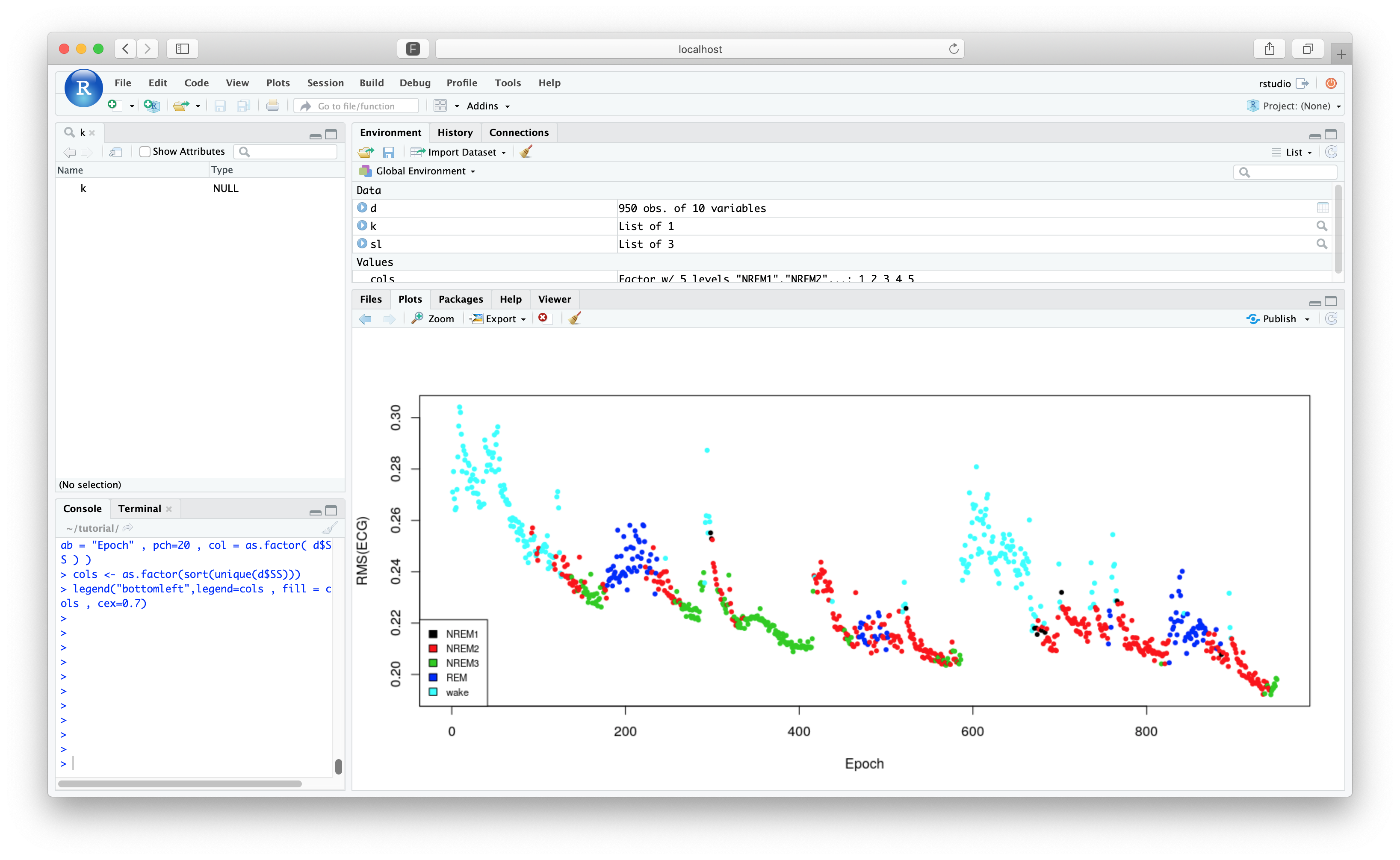
The aim is to plot the RMS of the ECG channel coloured by sleep stage.
To attach information on the sleep stage of an NSRR individual, we can
use the convenience function lstages():
d$SS <- lstages()
Note
As we can check, in this simple case we confirm that d is
exactly 1195 rows and ordered by epoch, and so we can use
lstages() (which returns a vector 1195 in length) to directly
populate a "sleep stage" variable. In practice, it is safer to
use the full results of leval("STAGE") (for which lstages() is
just a wrapper) and merge() based on E (or ID if necessary).
Following the previous tutorial section, we want to restrict the output to the first 950 rows (as the end of the recording contains artifact):
d <- d[ 1:950 , ]
plot( d$E , d$RMS , ylab = "RMS(ECG)" , xlab = "Epoch" , pch=20 , col = as.factor( d$SS ) )
cols <- as.factor(sort(unique(d$SS)))
legend("bottomleft",legend=cols , fill = cols , cex=0.7)
Hypnograms
Previous material
The corresponding section of the original tutorial covered:
- using
HYPNOto generate individual-level, cycle-level and epoch-level information about sleep architecture (based on manual staging)
Repeating these steps for nsrr01, we should first reset Luna's environment (just as a safety measure):
lreset()
lattach(sl,1)
lstages(), e.g. to get minutes in each stage:
table( lstages() ) / 2
   N1    N2    N3     R     W
 54.5 261.5   8.5 119.0 238.5
Running the HYPNO command for all three individuals:
k <- leval.project( sl , "HYPNO epoch" )
BL strata ):
d <- lx( k , "HYPNO" , "BL" )
Hint
If you're unsure about which strata and variables are
generated by a command, visit the its section in the
reference part of this website: they are
tabulated for every command. You can also run lx() (or destrat,
if on the command line).
To extract minutes of each stage for all individuals - these are stratified by sleep stage (SS):
d <- lx( k , "HYPNO" , "SS" )
d[ d$SS %in% c("N1","N2","N3","R") ,c("ID","SS","MINS")]
       ID SS  MINS
7  nsrr01 N1  54.5
8  nsrr02 N1   5.5
9  nsrr03 N1  26.0
10 nsrr01 N2 261.5
11 nsrr02 N2 199.5
12 nsrr03 N2 187.5
22 nsrr01 N3   8.5
23 nsrr02 N3  92.5
24 nsrr03 N3  10.5
28 nsrr01  R 119.0
29 nsrr02  R  60.0
30 nsrr03  R   0.0
Cycle-level and epoch-level output can be extracted with the commands:
d <- lx( k , "HYPNO" , "C" )
d <- lx( k , "HYPNO" , "E" )
Epoch-level masks
Previous material
The corresponding section of the original tutorial covered:
-
used epoch-level masks to select a particular subset of epochs for
nsrr01 -
illustrated how to attach epoch-level annotations after an EDF has been attached
The corresponding section aimed to select epochs that met the following criteria (made up simply to illustrate how the commands operate):
- epochs of persistent sleep (i.e. at least 10 minutes of sleep prior)
- that occur between 11pm and 3am
- and are during stage 2 NREM sleep
- and do not contain any apnea or hypopnea events
Although we could run cmd/third.txt as in the previous section, in
order to introduce some new lunaR commands, we'll do it a different
way. As before, if we've been doing previous work with lunaR, we
should first reset the environment:
lreset()
lattach( sl , 1 )
HYPNO command:
k <- leval( "HYPNO epoch" )
lx():
ps <- k$HYPNO$E$PERSISTENT_SLEEP
ps is a vector of 0 and 1 (i.e. no or yes) with as many elements as epochs for nsrr01:
table( ps)
ps
  0   1
720 644
In lunaR, we can attach a new annotation with either the
ladd.annot() or ladd.annot.file() command. The latter form can
read any Luna annotation format, i.e XML,
.annot or .eannot files. One option would be to save the
information about persistent sleep to a file, and load it with
ladd.annot.file() therefore. However, given we are already in R, it
is easier to just directly specify the annotation, using
ladd.annot(), which expects as input an R interval list. In this
context, an interval list is something in the format we get out of
the lannots() command for example.
We can use the helper function le2i() to convert epoch numbers to
intervals, given a particular definition of epoch duration (and
overlap), the default is 30 second, non-overlapping epochs. For example:
le2i( 1:4 )
> le2i( 1:10 )
[[1]]
[1]  0 30

[[2]]
[1] 30 60

[[3]]
[1] 60 90

[[4]]
[1]  90 120
ps==1):
ps.ints <- le2i( which( ps == 1 ) )
This gives a list ps.ints which is 384 elements long. We can add
this as a new annotation as follows (we assign the name
persistent_sleep but we could use anything):
ladd.annot( "persistent_sleep" , ps.ints )
We can check that it has been added as follows:
lannots()
 [1] "Arousal"           "Hypopnea"          "N1"
 [4] "N2"                "N3"                "Obstructive_Apnea"
 [7] "R"                 "SleepStage"        "SpO2_artifact"
[10] "SpO2_desaturation" "W"                 "persistent_sleep"
Finally, here we illustrate how to use multiple leval() statements
on the same attached EDF, to apply a series of masks (which could be
done in any order, in this example). Although this is always the
default, we can start by ensuring that all epochs are included
(i.e. none are masked):
leval( "MASK none" )
nsrr01 : 14 signals, 13 annotations, 11:22:00 duration, 1364 unmasked 30-sec epochs, and 0 masked
Next, we mask epochs not between 11pm and 3am:
leval( "MASK hms=23:00:00-03:00:00" )
nsrr01 : 14 signals, 13 annotations, 11:22:00 duration, 481 unmasked 30-sec epochs, and 883 masked
We see that the number of epochs has dropped from 1364 to 481
unmasked epochs. As previously noted,
we have 481 and not 480 (i.e. 4 hours) because the epochs start on 17
and 47 seconds past the minute in this particular EDF, and so we
include an additional epoch that starts at 10:59:47 but overlaps the
requested period. (Also note that, at this point, none have actually
been removed; that will not happen until a
RESTRUCTURE (or RE) command is
given.)
We next apply the persistent sleep mask:
leval( "MASK mask-ifnot=persistent_sleep" )
nsrr01 : 14 (of 14) signals, 12 annotations, 11:22:00 duration, 272 unmasked 30-sec epochs, and 1092 masked
leval( "MASK mask-ifnot=N2" )
nsrr01 : 14 (of 14) signals, 12 annotations, 11.22.00 duration, 235 unmasked 30-sec epochs, and 1129 masked
leval( "MASK mask-if=Obstructive_Apnea,Hypopnea" )
nsrr01 : 14 (of 14) signals, 12 annotations, 11.22.00 duration, 86 unmasked 30-sec epochs, and 1278 masked
We can confirm these steps by viewing the results of letable() and including these relevant annotations:
d <- letable( annots = c( "persistent_sleep" , "N2" , "Obstructive_Apnea" , "Hypopnea" ) )
We can view the epoch table here (if the image is too small, click to upon in a new browser tab):
View(d)
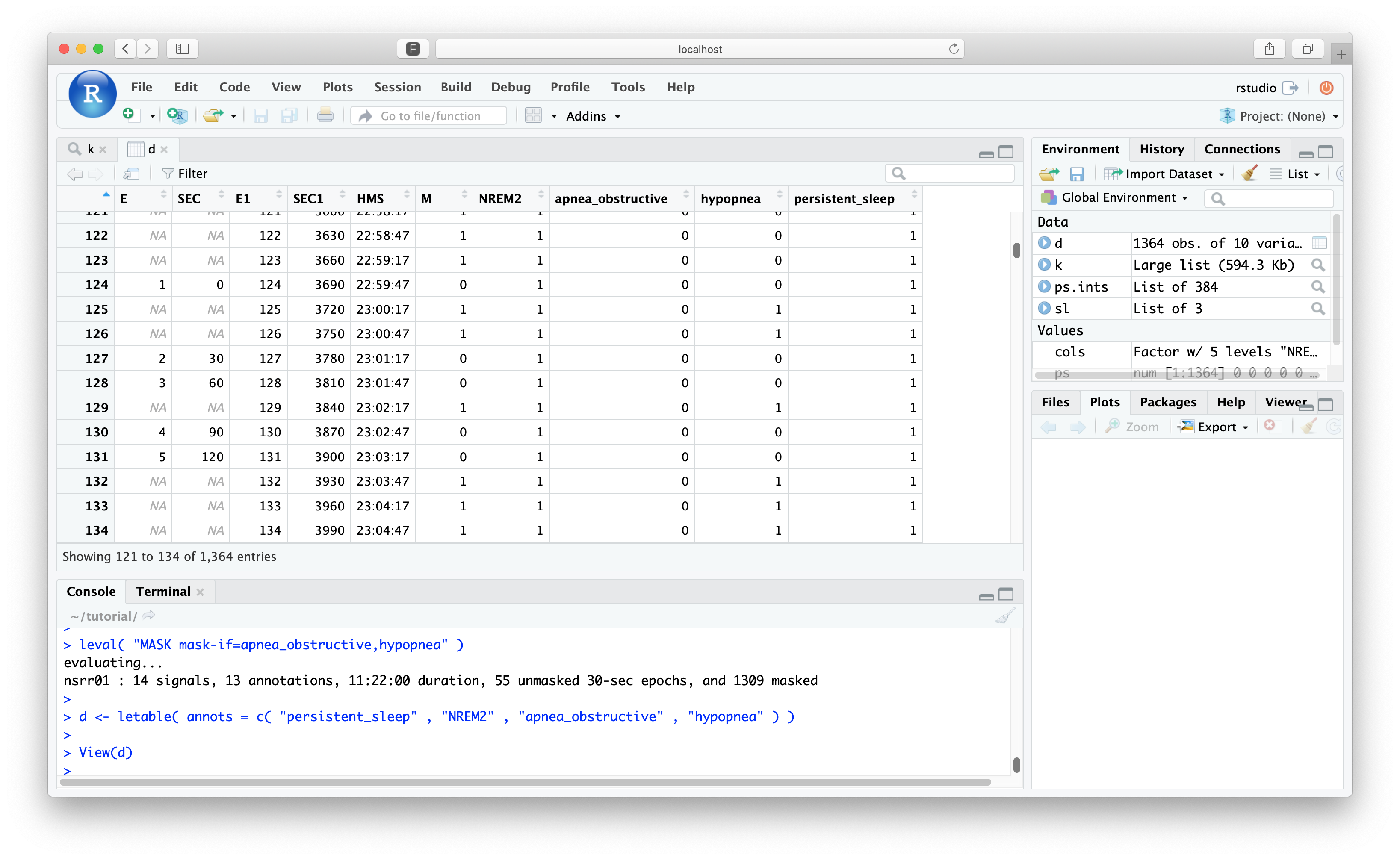
Epochs that are masked have M set to 1 and the epoch codes (E)
and start-time (SEC) are set to NA. Luna tracks the original
epoch numbers, start times and clock-time however (E0, SEC0 and
HMS). For example, the first epoch to be included (the new epoch #1) was the old epoch #124, etc.
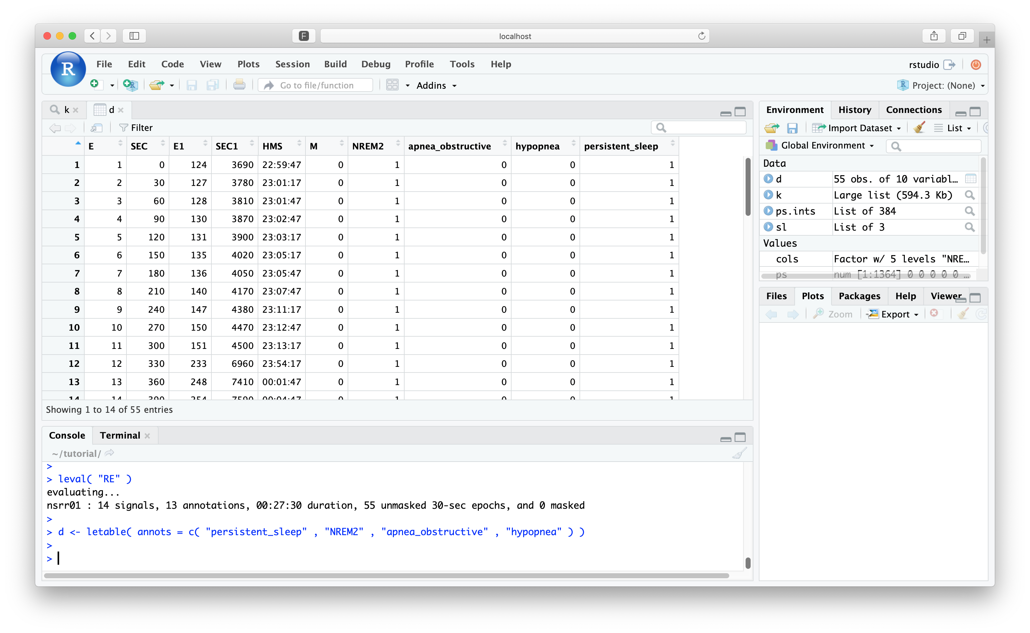
If we run a RESTRUCTURE command, all masked epochs are permanently dropped from the internal EDF, and so we'll
end up with a 86-epoch (43 minutes) dataset, but for which there are no masked epochs:
leval( "RE" )
nsrr01 : 14 (of 14) signals, 12 annotations, 00.43.00 duration, 86 unmasked 30-sec epochs, and 0 masked
Again, we can view the letable() for this:
d <- letable( annots = c( "persistent_sleep" , "N2" , "Obstructive_Apnea" , "Hypopnea" ) )
All masked epochs have now been dropped, although Luna still retains the original time/epoch encoding in E0, etc.
Manipulating EDFs
Previous material
The corresponding section of the original tutorial covered:
- filtering, resampling, relabeling and re-referencing signals
- re-writing new EDFs
The previous section basically involved running cmd/fourth.txt
through lunaC, which is as follows:
mV
RESAMPLE sr=100
FILTER bandpass=0.3,35 ripple=0.02 tw=1 fft
REFERENCE ref=EEG1 sig=EEG2
WRITE edf-tag=v2 edf-dir=newedfs/ sample-list=new.lst
luna s.lst @cmd/vars.txt sig=EEG1,EEG2 < cmd/fourth.txt
To mirror this, we first need to load the environment variables in the parameter file:
lset( "cmd/vars.txt" )
Next, we need to specify that only signals EEG1 and EEG2 (these
are aliases for EEG and EEG(sec)) be included:
lset( "sig" , "EEG1,EEG2" )
k <- leval.project( sl, lcmd( "cmd/fourth.txt" ) )
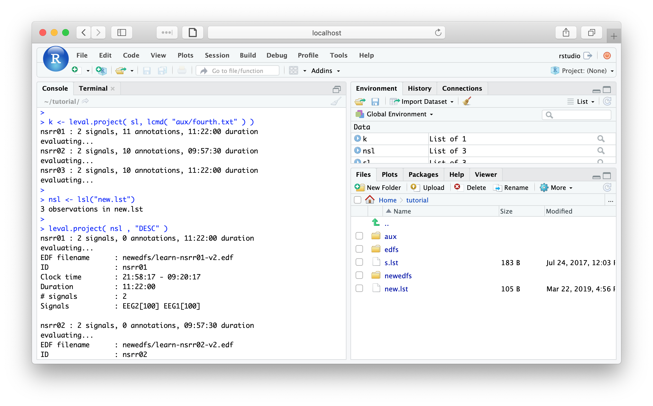
If you go the the Files tab in RStudio, you should be able to see
the newly created file and folder: new.lst and newedfs. We can
load this sample list, say calling is nsl for new sample-list:
nsl <- lsl("new.lst")
DESC command for all three individuals:
leval.project( nsl , "DESC" )
nsrr01 : 2 (of 2) signals, 0 annotations, 11.22.00.000 duration
evaluating...
EDF filename      : newedfs/learn-nsrr01-v2.edf
ID                : nsrr01
Clock time        : 21.58.17 - 09.20.17
Duration          : 11:22:00  40920 sec
# signals         : 2
Signals           : EEG2[100] EEG1[100]

nsrr02 : 2 (of 2) signals, 0 annotations, 09.57.30.000 duration
evaluating...
EDF filename      : newedfs/learn-nsrr02-v2.edf
ID                : nsrr02
Clock time        : 21.18.06 - 07.15.36
Duration          : 09:57:30  35850 sec
# signals         : 2
Signals           : EEG2[100] EEG1[100]

nsrr03 : 2 (of 2) signals, 0 annotations, 11.22.00.000 duration
evaluating...
EDF filename      : newedfs/learn-nsrr03-v2.edf
ID                : nsrr03
Clock time        : 20.15.00 - 07.37.00
Duration          : 11:22:00  40920 sec
# signals         : 2
Signals           : EEG2[100] EEG1[100]
Note
Annotation files are not automatically transferred to new EDFs, as currently Luna only writes EDF, not EDF+. As such, as timing information would be lost, if the EDF has been restructured.
Artifact detection
Previous material
The corresponding section of the original tutorial covered:
-
generating per-epoch statistics including RMS, Hjorth parameters and and index of signal-clipping
-
using these, alongside a second epoch-wise artifact detection algorithm based on spectral analysis, to flag likely aberrant epochs
-
visualizing these statistics across the night, and looking at raw EEG signals for an artifact-containing epoch
The corresponding section involved running cmd/fifth.txt to generate
the above-mentioned statistics, and then a slightly modified version
(cmd/sixth.txt) to actually mask potentially bad epochs, all for nsrr01.
Reset the Luna environment:
lreset()
Before attaching the EDF, we can specify that we want to restrict
analyses to the EEG channel (no other variables were used in this
script, so we didn't attach a parameter file, and so we use EEG and
not the alias EEG1 here):
lset( "sig" , "EEG" )
Attach nsrr01:
lattach( sl , 1 )
Run the script:
k <- leval( lcmd( "cmd/fifth.txt" ) )
lx( k , "SIGSTATS" , "CH" )
      ID  CH       H1        H2        H3
1 nsrr01 EEG 78.38342 0.3536182 0.8316128
Extract epoch-level statistics:
d <- lx( k , "SIGSTATS" , "CH" , "E" )
We can now tabulate:
View(d)
q <- leval( "STAGE" )
> ss <- lx(q,"STAGE")
> head(ss)
      ID  E CLOCK_TIME MINS OSTAGE STAGE STAGE_N START
1 nsrr01 54   22:24:47 26.5     N1    N1      -1  1590
2 nsrr01 55   22:25:17 27.0     N1    N1      -1  1620
3 nsrr01 56   22:25:47 27.5     N1    N1      -1  1650
4 nsrr01 58   22:26:47 28.5     N1    N1      -1  1710
5 nsrr01 59   22:27:17 29.0     N1    N1      -1  1740
6 nsrr01 60   22:27:47 29.5     N1    N1      -1  1770
> dim(ss)
[1] 887   8
> dim(d)
[1] 887   6
m <- merge( d , ss , by="E" )
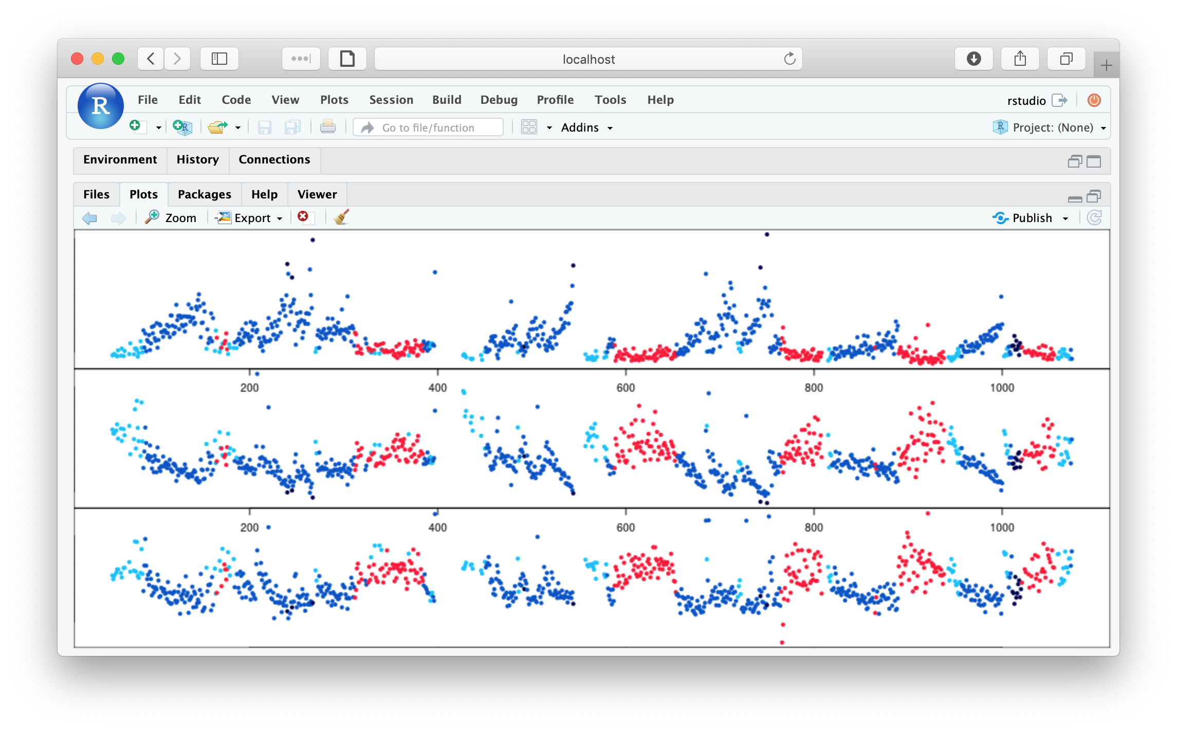
par(mfcol=c(3,1),mar=c(0,0,0,0))
plot( m$E , m$H1 , pch=20 , col = lstgcols( m$STAGE ) )
plot( m$E , m$H2 , pch=20 , col = lstgcols( m$STAGE ) )
plot( m$E , m$H3 , pch=20 , col = lstgcols( m$STAGE ) )
As well as clear evidence of ultradian dynamics (that correspond to sleep stage), we see evidence of some outlier epochs in these plots (Hjorth parameters 1, 2 and 3 from top to bottom):
We'll now run the slightly modified script, that masks outlier epochs based on these metrics.
EPOCH
MASK if=W
RESTRUCTURE
FILTER bandpass=0.3,35 ripple=0.02 tw=1
SIGSTATS epoch
ARTIFACTS mask
CHEP-MASK ep-th=3,3,3
CHEP epochs
DUMP-MASK
See ARTIFACTS and
CHEP-MASK for details.
Because the previous cmd/fifth.txt script modified the internal EDF, we need to reattach or refresh it:
lrefresh()
nsrr01 : 1 signals, 11 annotations, 11:22:00 duration
We don't need to lreset() as we want to keep the same sig
environment variable. Because sig is still set, when re-attaching
we only load that single channel (i.e. it's not that lrefresh()
didn't work somehow here, as by itself would have led to in all
channels being read in).
Running this new script:
k <- leval( lcmd( "cmd/sixth.txt" ) )
nsrr01 : 1 signals, 11 annotations, 07:23:30 duration, 840 unmasked 30-sec epochs, and 47 masked
It appears from the above that 47 sleep epochs have been masked on the
basis of epoch-level artifact detection. We can look at the EMASK variable in the
epoch-level output from the DUMP-MASK command:
d <- k$DUMP_MASK$E
table( d$EMASK )
  0   1
840  47
To see which epochs are masked:
head( d[ d$EMASK == 1 , ])
       ID   E   EMASK
14 nsrr01  78       1
16 nsrr01  80       1
20 nsrr01  85       1
24 nsrr01  89       1
80 nsrr01 145       1
81 nsrr01 146       1
Hint
In lunaR, we could also use the letable() function to look at the current mask status:
table( letable()$M )
  0   1
840  47
Finally, to plot the Hjorth parameter statistics visually indicating which are masked:
h <- lx( k , "SIGSTATS" , "CH" , "E" )
m <- merge( d , h , by="E" , all = T )
To obtain the same plot: Hjorth parameters per epoch with a flag to indicate a mask
par(mfcol=c(3,1),mar=c(4,4,1,1))
plot( m$E , m$H1 , pch = 20 , xlab="Epoch" , ylab="H1" , col = m$EMASK + 1)
plot( m$E , m$H2 , pch = 20 , xlab="Epoch" , ylab="H2" , col = m$EMASK + 1)
plot( m$E , m$H3 , pch = 20 , xlab="Epoch" , ylab="H3" , col = m$EMASK + 1)
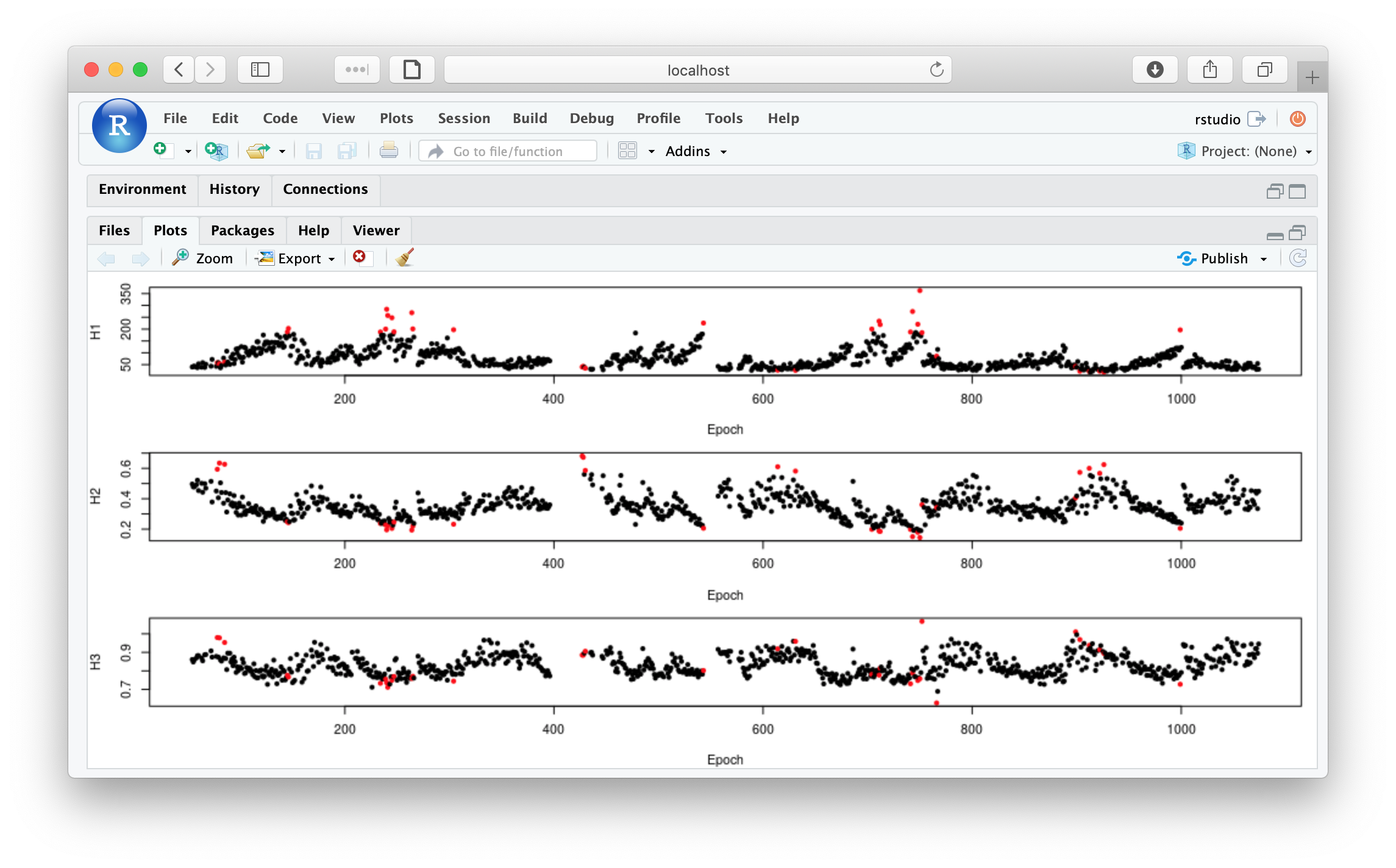
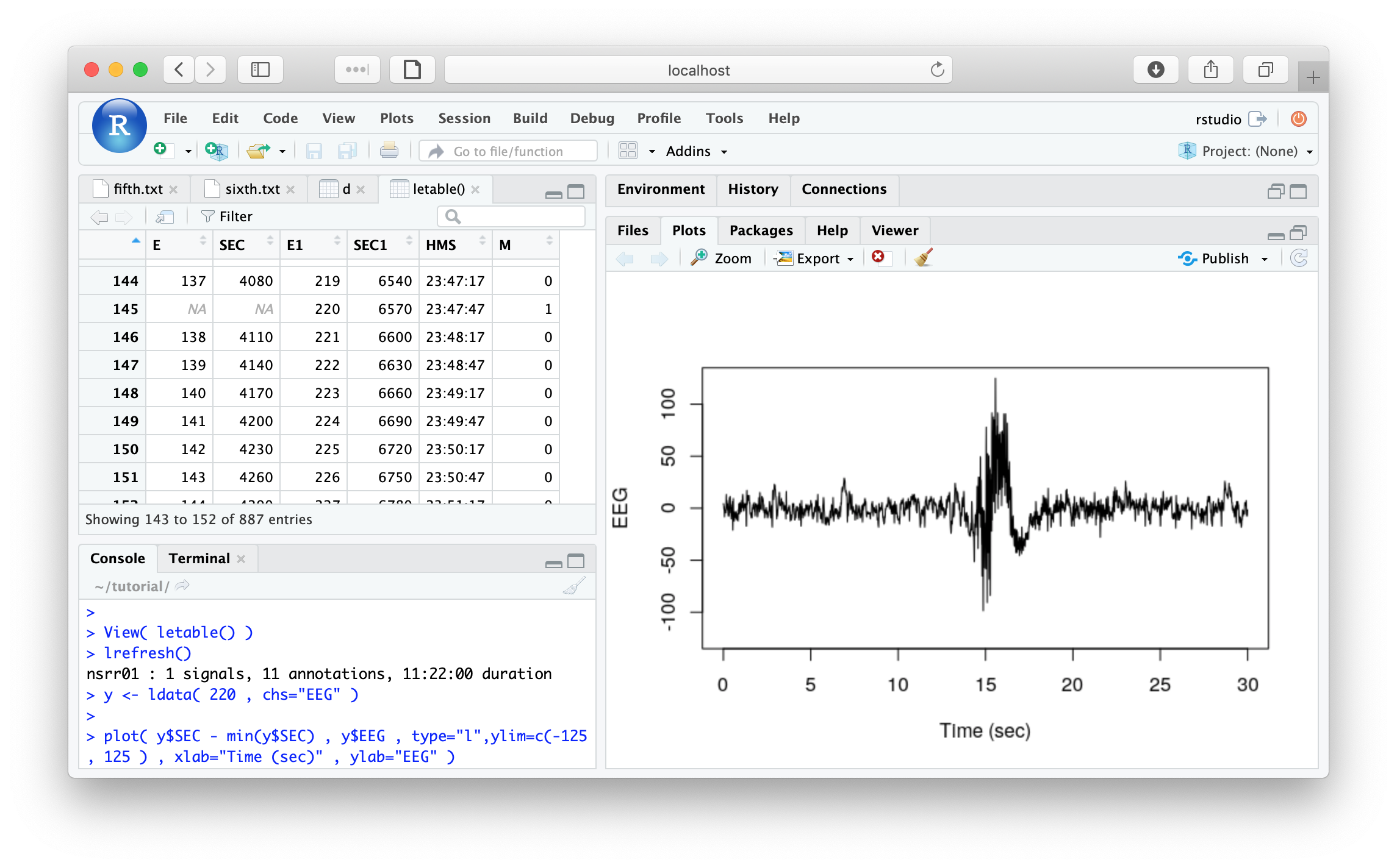
From looking at d, we see that epoch #220 is one of the masked
epochs. To view it, we can use the ldata() function. Naturally, we
first need to refresh the EDF or clear the mask (i.e. as it is currently masked):
lrefresh()
y <- ldata( 220 , chs="EEG" )
plot( y$SEC - min(y$SEC) , y$EEG , type="l",
      ylim=c(-125, 125 ) , xlab="Time (sec)" , ylab="EEG" )
Spectral and spindle analyses
Previous material
The corresponding section of the original tutorial covered:
-
estimating power spectra for cleaned and raw EEG signals for all three tutorial individuals
-
additionally detecting fast and slow spindles
In this final section, we'll re-run the cmd/seventh.txt script in lunaR:
EPOCH
MASK ifnot=N2
RESTRUCTURE
FILTER bandpass=0.3,35 ripple=0.02 tw=1 fft
ARTIFACTS mask
CHEP-MASK ep-th=3,3,3
CHEP epoch
RESTRUCTURE
PSD spectrum
SPINDLES fc=11,15 annot=spindles
WRITE-ANNOTS file=spindles-^.txt annot=spindles
We'll first reset all environment variables:
lreset()
lstat()
Error in lstat() : no EDF attached
We'll reload the original set of environment variables we've been using:
lset( "cmd/vars.txt" )
lset( "sig" , "EEG1" )
k <- leval.project( sl , lcmd( "cmd/seventh.txt" ) )
We can extract the PSD (which is stratified by channel and frequency):
d <- lx( k , "PSD" , "CH" , "F" )
For the plot, to mirror the previous tutorial, we'll restrict the plot to frequencies of 0.5 Hz and above:
d <- d[ d$F >= 0.5 , ]
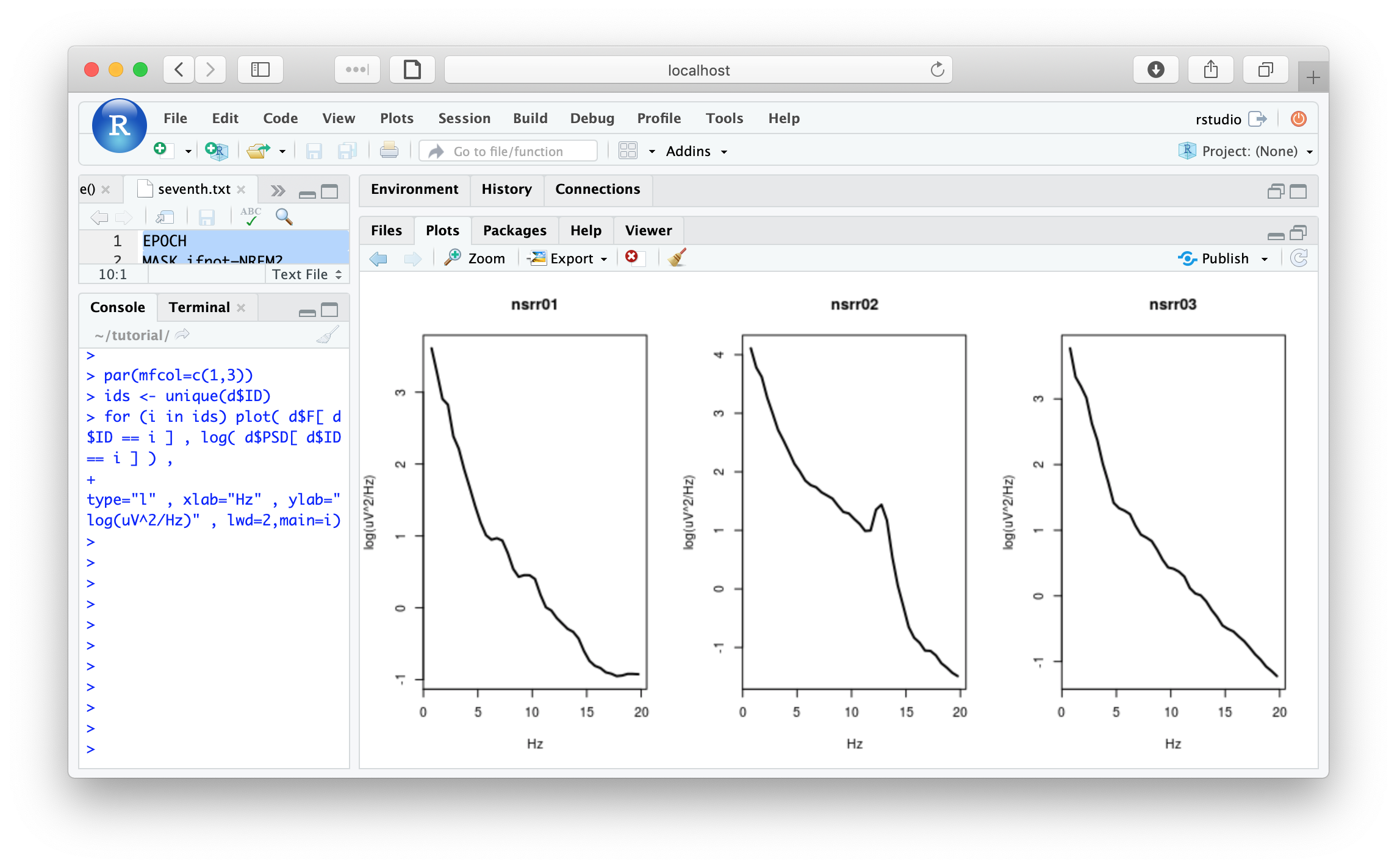
Plots of power spectra; create 3 plots, on a log-scale (nb. due to very minor changes in some of the default settings of Luna since making this plot, the exact contour of these PSDs may look slightly different from below):
par(mfcol=c(1,3))
ids <- unique(d$ID)
for (i in ids) plot( d$F[ d$ID == i ] , log( d$PSD[ d$ID == i ] ) ,
  type="l" , xlab="Hz" , ylab="log(uV^2/Hz)" , lwd=2,main=i)
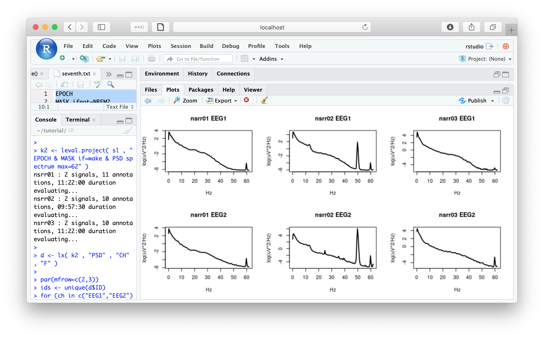
Next, mirroring the previous tutorial section, we need to repeat the PSD estimation, now for both channels and without the band-pass filtering or artifact detection steps, and also showing the full spectra (up to close to the Nyquist frequency);
We can append the channel aliased by EEG2 to the signal list (i.e. EEG1 will remain):
lset( "sig" , "EEG2" )
We can specify the Luna commands on the R command line this time, instead of reading them from a file:
k2 <- leval.project( sl , "EPOCH & MASK if=W & PSD spectrum max=62" )
Extracting the PSD:
d <- lx( k2 , "PSD" , "CH" , "F" )
par(mfrow=c(2,3))
ids <- unique(d$ID)
for (ch in c("EEG1","EEG2") )
 for (i in ids)
   plot( d$F[ d$ID == i & d$CH == ch ] , log( d$PSD[ d$ID == i & d$CH == ch ] ) ,
            type="l" , xlab="Hz" , ylab="log(uV^2/Hz)" , lwd=2,main=paste(i,ch))
Now we'll turn to the spindle detection that was performed as part of cmd/seventh.txt.
As described here, the primary individual-level output of
SPINDLES if stratified by channel (CH) and target frequency (F):
d <- lx( k , "SPINDLES" , "F" , "CH" )
DENS):
d[ , c("ID","CH","F","DENS") ]
      ID   CH  F      DENS
1 nsrr01 EEG1 11 0.7300971
2 nsrr02 EEG1 11 1.2860759
3 nsrr03 EEG1 11 0.7242340
4 nsrr01 EEG1 15 0.6407767
5 nsrr02 EEG1 15 2.0556962
6 nsrr03 EEG1 15 0.1949861
We've now completed the steps of the previous lunaC tutorial. As
mentioned elsewhere, lunaC is likely a better tool for running
analyses on a large number of studies. The advantages of lunaR are
primarily in terms of being able to leverage the power of the R
language and its graphical abilities. Along these lines, we'll close
by using lunaR to visualize the spindles detected on nsrr02, which
also illustrates some additional lunaR functions.
We'll focus on nsrr02, in part because the other two studies had
relatively low rates of spindles detected. This is not necessarily
unusual in older subjects, who may have fragmented sleep and/or
full-blown sleep disorders. The presence of artifact can also
influence rates of spindles detected, of course, and so a more careful
analyses and inspection of the data would be required before making
any strong conclusions about these data.)
We'll restrict analyses to EEG1, by first reseting the signal list and then adding EEG1:
lset( "sig", "." )
lset( "sig" , "EEG1" )
lattach( sl ,2 )
nsrr02 : 1 signals, 10 annotations, 09:57:30 duration
Re-running the script cmd/seventh.txt for this one individual
(i.e. using level() and not leval.project()):
k <- leval( lcmd( "cmd/seventh.txt" ) )
Hint
If you get errors such as
Error in leval(lcmd("cmd/seventh.txt")) :
   problem flag set: likely no unmasked records left? run lrefresh()
lset(); if in doubt, running lreset(),
lrefresh() and repeating the commands is always a good idea.
Also, using lchs() and lstat() can help to orient you, in
terms of what has been "done" to the in-memory EDF since it was
attached.
lx(k)
ARTIFACTS : CH
EPOCH : BL
MASK : EMASK
PSD : CH B_CH CH_F
RESTRUCTURE : BL
SPINDLES : CH_F CH_F_SPINDLE
We can extract the time-points from the SPINDLES table that is
stratified by SPINDLE as well as CH and F (i.e. the
spindle-level results):
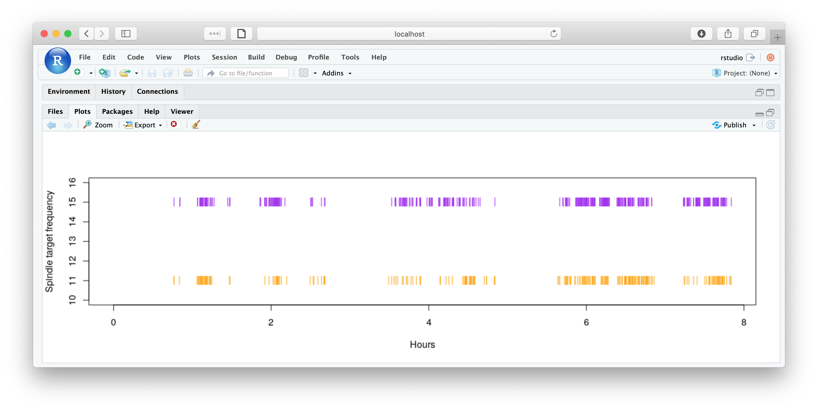
d <- lx( k , "SPINDLES" , "CH_F_SPINDLE" )
table( d$F )
 11  15
254 406
In other words, we detected 406 fast (15 Hz) spindles and 254 slow (11
Hz) spindles. That variable START (and START_SP) reflects the
time in seconds (and in sample-points based on the current internal
EDF) on when each spindle started; STOP variables are similarly
defined.
We can plot when the spindles occur, as follows (nb. obviously there are many ways to do this and this isn't necessarily to most elegant or visually informative...)
d11 <- d[ d$F == 11 , ]

d15 <- d[ d$F == 15 , ]

plot( d11$START/3600 , rep( 11, length(d11$START) ) ,
  pch="|" , ylim=c(10,16), col="orange",xlim=c(0,max(d$START)/3600),
  xlab="Hours", ylab="Spindle target frequency" )

points( d15$START/3600 , rep( 15, length(d15$START) ) ,
  pch="|" , ylim=c(10,16), col="purple")
The annot option we used for the SPINDLES command means that
Luna will have written an .annot file to the
edfs/ folder. We can load those annotation files in as new annotations
to be attached to the current EDF.
ladd.annot.file( "spindles-nsrr02.txt" )
Now, when we ask for a list of attached annotations, we'll see a new one, spindles:
lannots()
 [1] "Arousal"           "Hypopnea"          "N1"
 [4] "N2"                "N3"                "Obstructive_Apnea"
 [7] "R"                 "SpO2_artifact"     "SpO2_desaturation"
[10] "W"                 "spindles"
We'll then use the lannots() function with a annotation class name
specified, to get a list of intervals for that annotation:
sp.intervals <- lannots( "spindles" )
This list is 660 elements in length, i.e. corresponding to the 998 spindles detected above:
length(sp.intervals)
[1] 660
Taking a peak at the contents of sp.intervals, we see each item is a
pair of numbers: the start and stop of the spindles in elapsed seconds
(from the EDF start time):
head( sp.intervals )
[[1]]
[1] 2751.304 2751.896

[[2]]
[1] 2764.040 2764.592

...
Now let's take a look at some spindles in the raw EEG. The
ldata.intervals() command will pull out the raw signal data (and
optionally other annotations) for one or more intervals. Optionally,
we can also specify a window (in seconds) around each annotation
interval. Here we specify 5 seconds (w=5), meaning that this function
will return the raw signal corresponding to a spindle interval, plus
and minus 5 seconds. (If the EDF is discontinuous, i.e. due to
masking and restructuring, or if the interval abuts the start or end
of the recording, this window will be shortened as appropriate.)
Here, we request the raw signal data from the channel with alias
EEG1 as well as the annotation channel sp.label (i.e. fast
spindles). The first argument indicates which interval(s) we want to
look at -- for simplicity, here we'll request a single spindle, say
the 221st, with sp.intervals[221]:
d <- ldata.intervals( sp.intervals[ 221 ], chs="EEG1", annots= "spindles", w=5 )
Looking at the d data frame returned by ldata.intervals():
head(d)
                 INT      SEC       EEG1 spindles
1 15129.87->15140.66 15129.87 -11.184889        0
2 15129.87->15140.66 15129.88 -10.571929        0
3 15129.87->15140.66 15129.89 -11.300724        0
4 15129.87->15140.66 15129.90  -9.616291        0
5 15129.87->15140.66 15129.90  -5.364184        0
6 15129.87->15140.66 15129.91  -3.394990        0
The annotation field (final column) is 0 or 1 to indicate the
presence or absence of that annotation (i.e. a fast spindle) at that
sample-point.
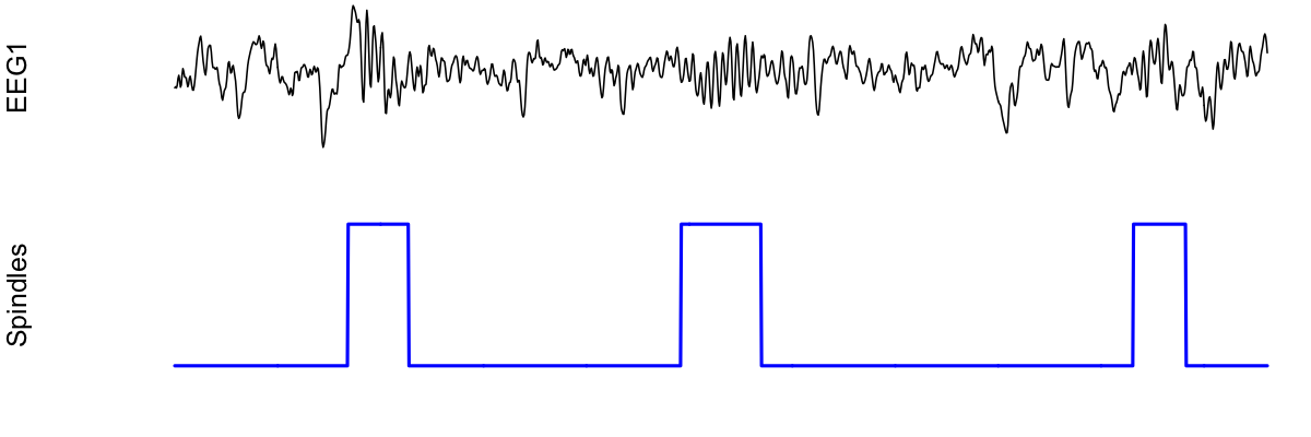
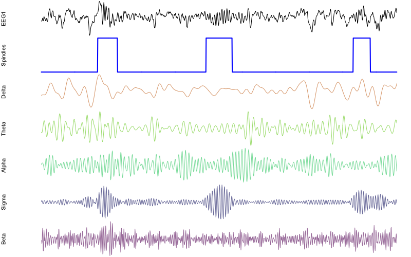
To plot this spindle, we could use something like the following:
par(mfcol=c(2,1) , mar=c(2,4,0,0) )
plot( d$EEG1 , type="l" , xaxt = 'n' , yaxt='n' , axes=F , ylab="EEG1" )
plot( d[, "spindles" ] , type="l" , lwd=2 , col="blue" , xaxt='n' , yaxt='n' , axes=F, ylab="Spindles" )
So far, so good. Let's extend this to show some other information in
the plot: say, band-pass filtered versions of the original EEG signal.
We'll use the same approach as shown in the example for the
FILTER command, whereby we made five
or so copies of a channel, and then band-pass filtered each copy to
correspond to delta, theta, alpha, sigma and beta power. In fact,
lunaR has a convenience function that does this automatically,
lbands(), which takes a channel names and creates five new channels
that are the band-pass filtered versions. Running it with the
nsrr02 EDF still attached (actually, at this point the in-memory
representation will reflect a masked and filtered version of EEG1
for NREM2 sleep only):
lbands( "EEG1" )
If we look at the list of channels present, we should now see the following new channels (these are not saved to the on-disk EDF, rather they exist only in the in-memory representation):
lchs()
[1] "EEG1"       "EEG1_delta" "EEG1_theta" "EEG1_alpha" "EEG1_sigma"
[6] "EEG1_beta"
We can now re-run the ldata.intervals() function, but this time
requesting all of these channels to be included in the output, by
setting chs equal to lchs() (i.e. all channels):
d <- ldata.intervals( sp.intervals[ 221 ], chs=lchs(), annots="spindles" , w=5 )
Run head(d) to confirm the structure of the new output. We can now
augment the plotting code to include these additional channels:
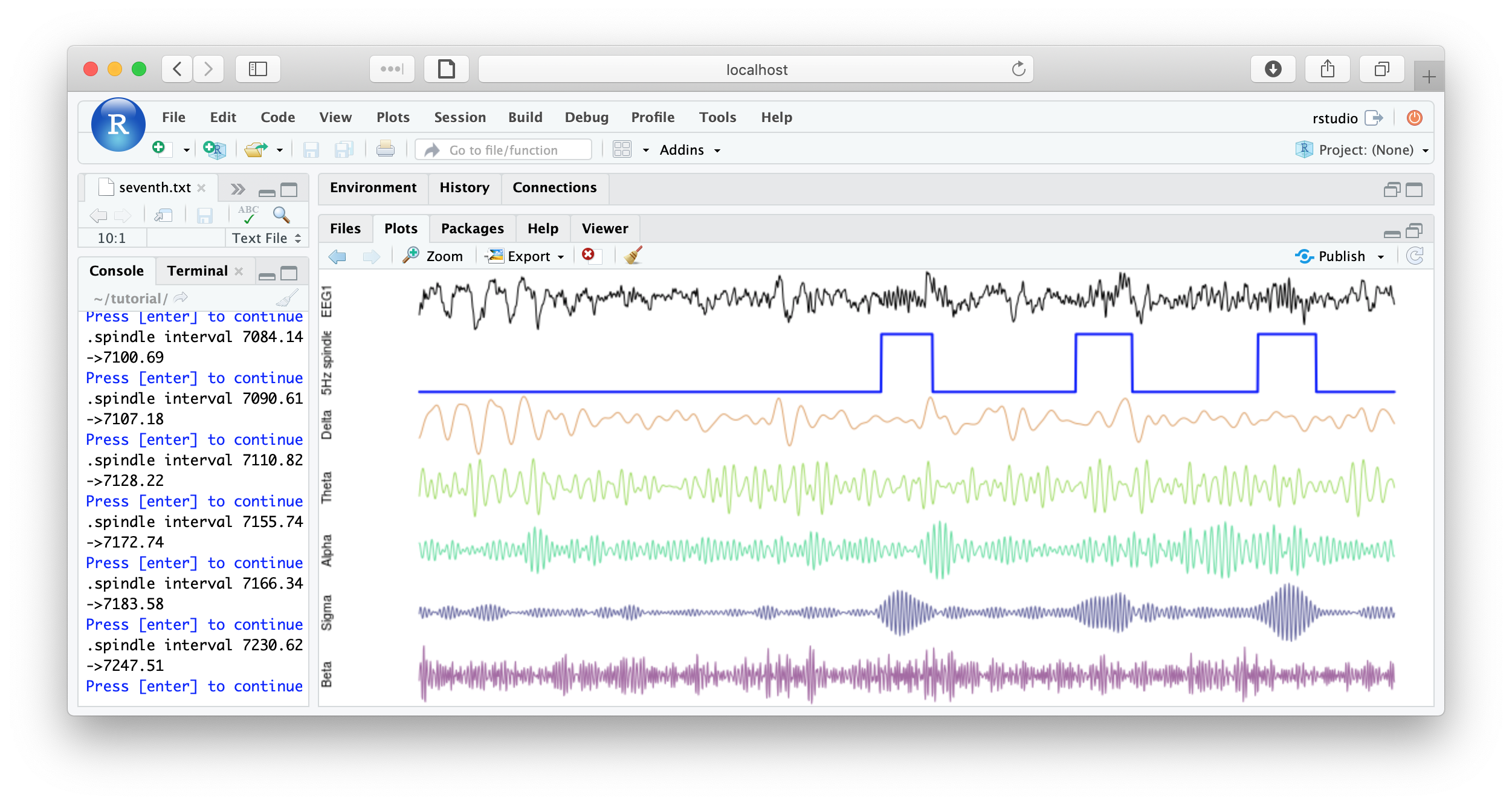
png(file="rt21.png",res=100,width=800,height=500,units="px")
par(mfcol=c(7,1) , mar=c(0,4,0,0) )
plot( d$EEG1 , type="l" , xaxt = 'n' , yaxt='n' , axes=F , ylab="EEG1" )
plot( d[, "spindles" ] , type="l" , lwd=2 , col="blue" , xaxt='n' , yaxt='n' , axes=F, ylab="Spindles" )
plot( d$EEG1_delta , type="l" , col=rgb(200,100,00,150,max=255) , axes=F , ylab="Delta" )
plot( d$EEG1_theta , type="l" , col=rgb(100,200,0,150,max=255) , axes=F , ylab="Theta" )
plot( d$EEG1_alpha , type="l" , col=rgb(0,200,100,150,max=255) , axes=F , ylab="Alpha" )
plot( d$EEG1_sigma , type="l" , col=rgb(0,0,100,150,max=255) , axes=F , ylab="Sigma" )
plot( d$EEG1_beta  ,  type="l" , col=rgb(100,0,100,150,max=255) , axes=F , ylab="Beta" )
dev.off()
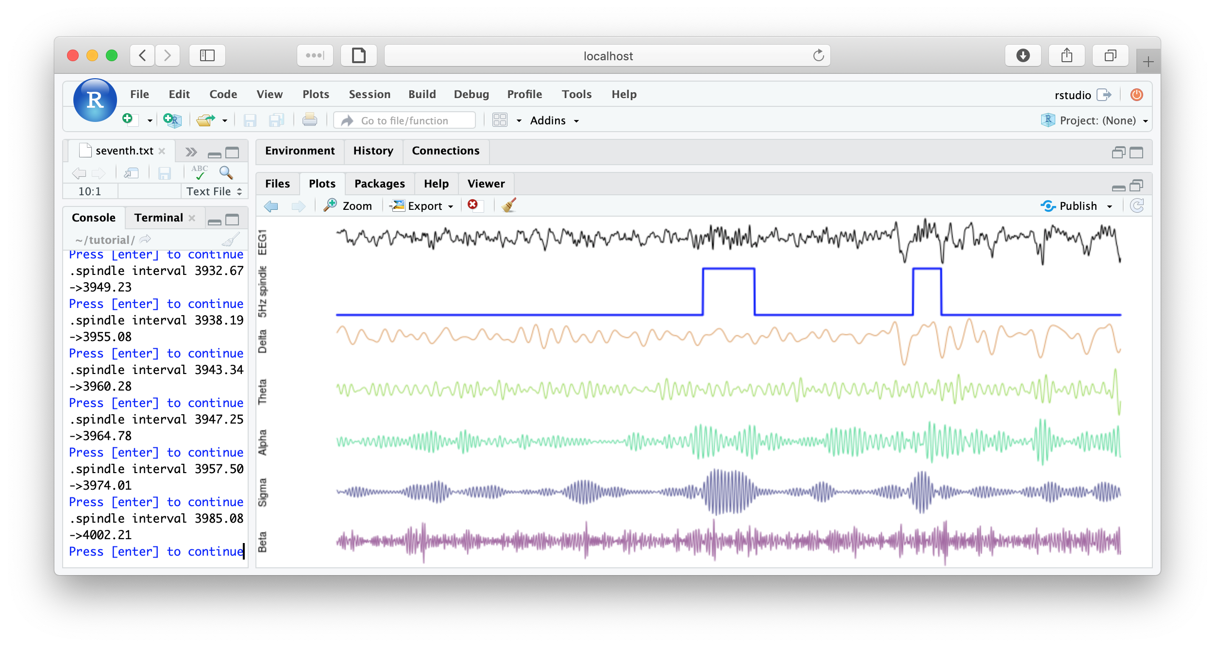
In practice, there would be few scenarios where one wants to extract particular spindles
for visaulization, beyond didactic purposes. To make this a little more useful,
rather than having to manually re-run this code for each
spindle, we can use Luna's literate() function to automate this
process. Given a list of intervals (or epoch-by-epoch), literate()
will iterate over each one, generate a data frame (by calling either
ldata.intervals() or ldata()) and then pass that data-frame to a
user-defined function. We'll wrap our plotting code in a function
(f1()) as follows:
f1 <- function(d) {
 par(mfcol=c(7,1) , mar=c(0,4,0,0) )
 plot( d$EEG1 , type="l" , xaxt = 'n' , yaxt='n' , axes=F , ylab="EEG1" )
 plot( d$spindles   , type="l" , lwd=2 , col="blue" , xaxt='n' , yaxt='n' , axes=F, ylab="Spindles" )
 plot( d$EEG1_delta , type="l" , col=rgb(200,100,00,150,max=255) , axes=F , ylab="Delta" )
 plot( d$EEG1_theta , type="l" , col=rgb(100,200,0,150,max=255) , axes=F , ylab="Theta" )
 plot( d$EEG1_alpha , type="l" , col=rgb(0,200,100,150,max=255) , axes=F , ylab="Alpha" )
 plot( d$EEG1_sigma , type="l" , col=rgb(0,0,100,150,max=255) , axes=F , ylab="Sigma" )
 plot( d$EEG1_beta  ,  type="l" , col=rgb(100,0,100,150,max=255) , axes=F , ylab="Beta" )
 cat( "spindle interval" , d$INT[1] , "\n" )
 readline(prompt="Press [enter] to continue")
}
That is, this is identical to the prior plotting code, simply inside a
function that also prints the spindle interval to the console, and
requests that the [enter] key be pressed to advance to the next
spindle. We can then instruct lunaR to iterate over the annotation
class spindles (with by.annot), which will create a data-frame
similar to the ones above for each spindle, plus or minus 8 seconds in
this case (w=8), and then pass it to the newly-defined f1() function:
literate( f1 , chs= lchs() , annots= "spindles" , by.annot= "spindles" , w = 8 )
Warning
The current implementation of literate() can lead to issues if
the function returns and error or is interupted (or may give issues by not allowing an interupt, e.g. from Ctrl-C, Ctrl-Z or similar):
this should be fixed on the next release... for now, treat literate() with care...
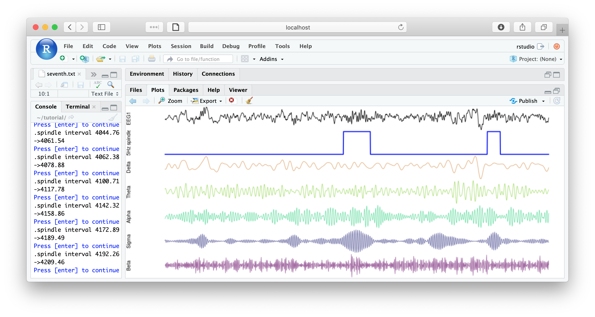
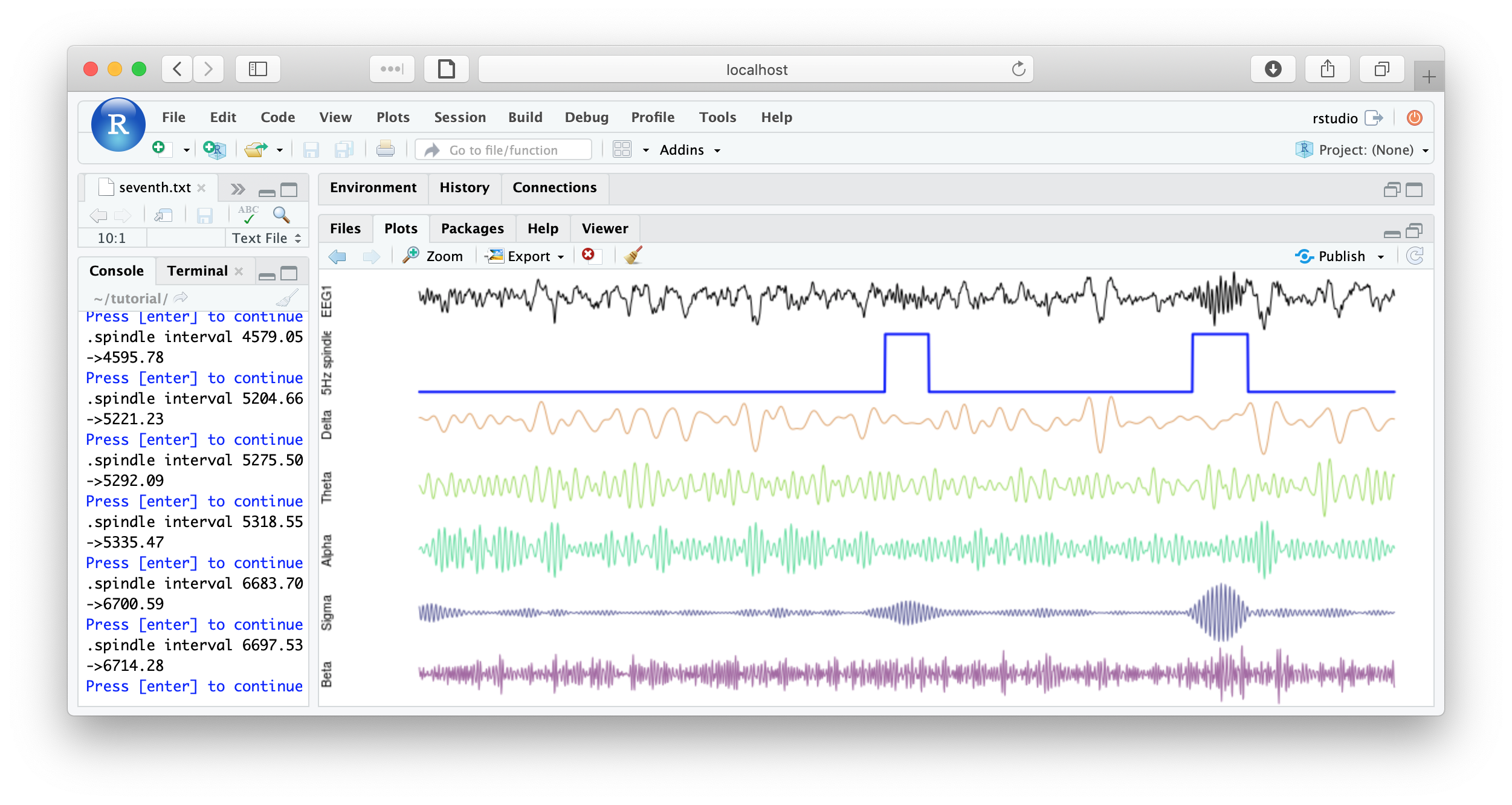
You could imagine adding some code to save each plot, or to make multiple plots per page, etc, for reviewing all spindles detected. Some example below:
That's the end of the tutorial. If this was your first pass, that was likely a lot of material to cover. Consult the command reference for more details about specific commands. And visit these pages for more details on using lunaC and lunaR.
Feel free to explore the tutorial data more -- as with any dataset, there are probably a few quirks that you might discover if you look closely enough. Have fun -- and if you get tired, remember you can always sleep on it and you'll probably understand it better the next day :-)