Visualizing the NSRR with UMAP

Uniform Manifold Approximation and Projection (or UMAP) is a new dimension reduction technique that can be used to visualize patterns of clustering in high-dimensional data. Unlike PCA (but similar to other approaches such as t-SNE), it is focused on local clustering, meaning that whilst "similar" observations should be grouped together, it does not attempt to preserve the exact global structure between all observations. Seemingly, in many contexts this property can make for more intuitive (and visually interesting) representations of data. (Think of sorting Lego blocks into piles based on their shape and size: you'd likely only care that similar blocks are in the same pile, and not about the relative positions of the different piles to each other.)

This approach has been used widely on single-cell RNA sequencing data to delineate cell types, as well as population genetic data, to reveal fine scale ethnic and geographical structure in human populations at different scales. And, conveniently, UMAP is very computationally efficient.

Sounds great -- so what does the NSRR look like through the lens of UMAP?

Purely to explore some NSRR data and to generate a few images for their own sake, we applied UMAP (as implemented in the umap R package and making absolutely no effort to use anything other than its default settings) to EEG power spectra from over 10 million epochs of sleep.

The data

We considered nine NSRR datasets: CHAT (baseline and follow-up datasets), CCSHS, CFS, SHHS (waves 1 and 2), MESA, MrOS and SOF. We extracted all sleep epochs (30-second epochs, based on NSRR's manual staging), removing epochs with any manually-annotated arousal or gross artifact. We then estimated the power spectral density (PSD) for the C4-M1 EEG channel for every epoch. In total, this analysis calculated power spectra for 10,389,017 epochs in 16,722 individuals. Parallelizing jobs on a compute cluster, the Luna analyses took about 1.5 hours to run.

Clustering individuals

As a broad initial sanity-check, we first considered the average power spectra per cohort, for all sleep epochs (i.e. merging both REM and NREM). After removing outliers, we obtained the following:

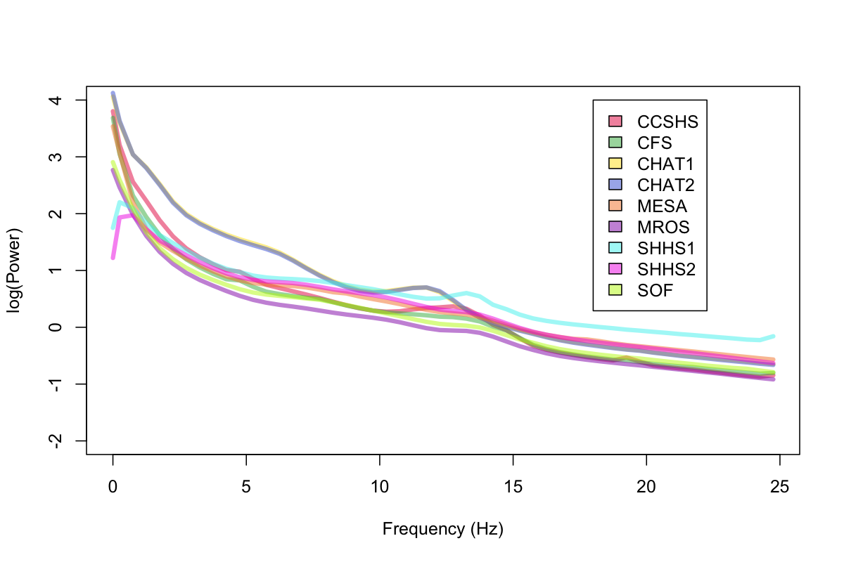
The PSD of the two CHAT studies (which are studies of younger children) almost completely overlap (these are the two lines with the highest theta power, although they look like a single line because of the overlap). Also of note: we can see bumps in the sigma range for a number of studies (bearing in mind here we've averaged over REM as well as NREM epochs). We can also see that SHHS1 and SHHS2 seem to have had low-frequency activity filtered out at the hardware level (as we did not apply any bandpass or high-pass filtering for these analyses). In any case, these spectra look broadly as expected.

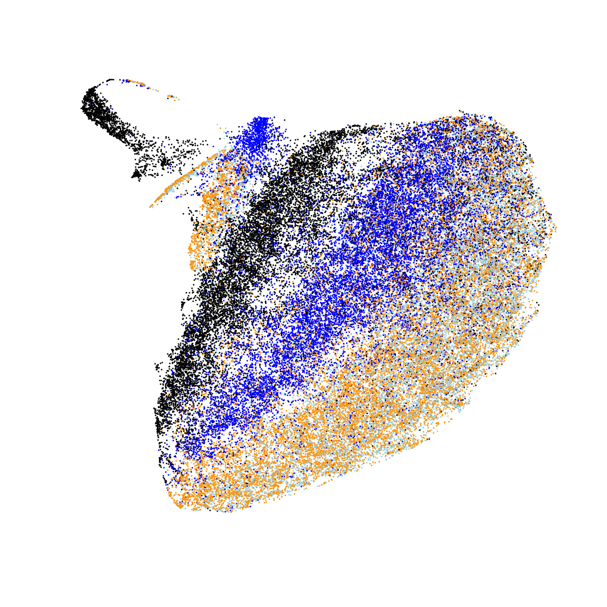
Using each individual's average absolute log-scaled power spectra as the input to UMAP for dimension reduction, this is a snapshot of the "NSRR sleep EEG". Each point represents a single individual, with the colors indicating the cohort:

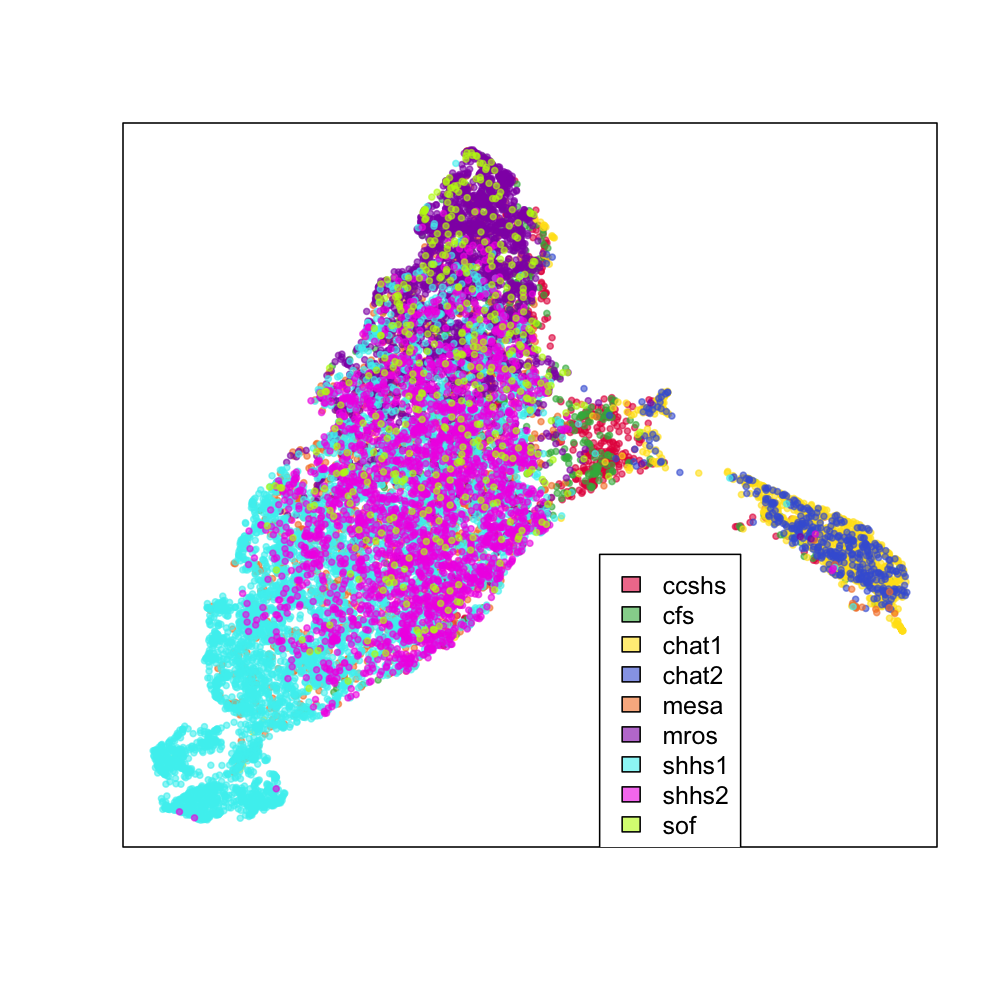
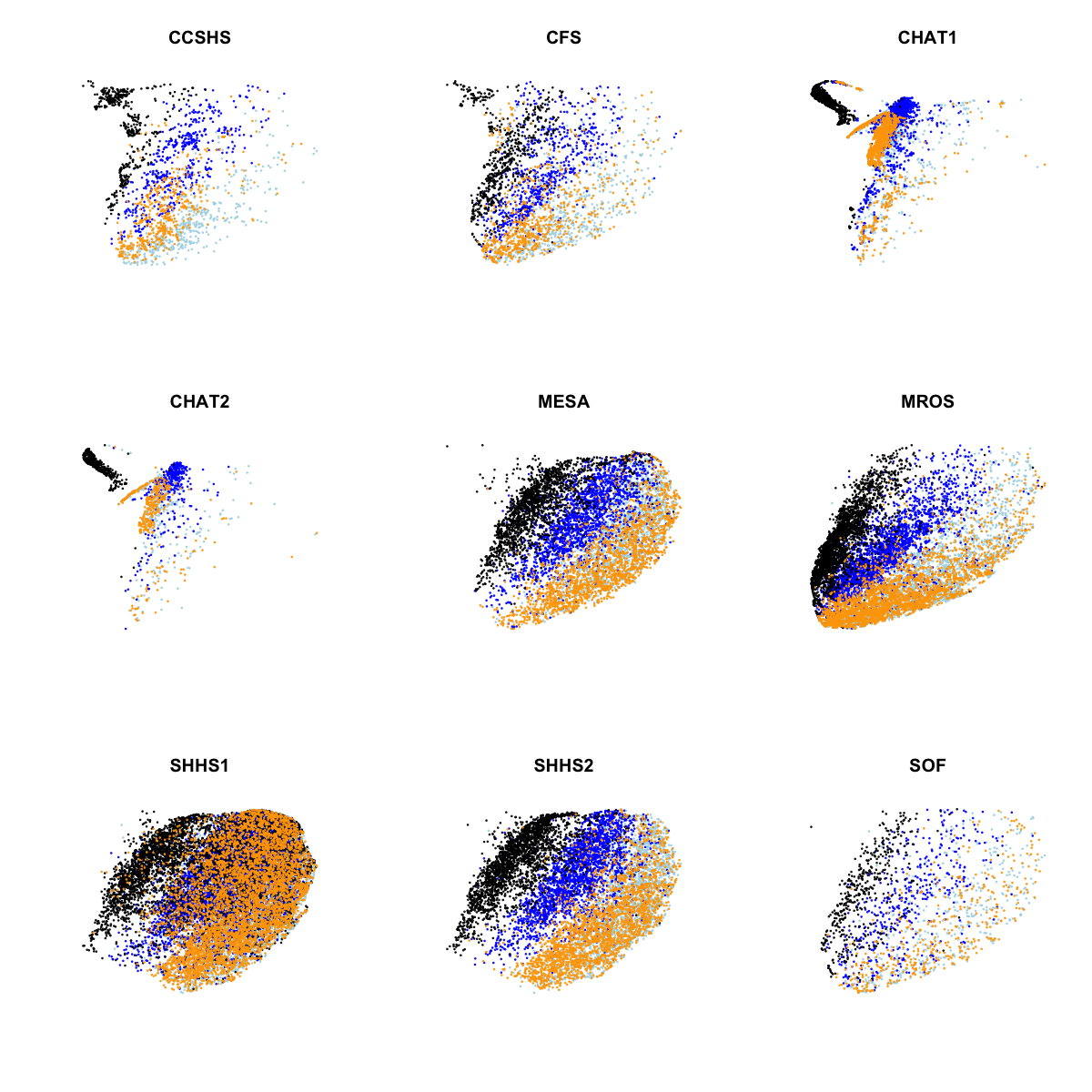
We see the two CHAT studies (blue and yellow) form their own cluster, but otherwise most individuals fall into a single large cluster. There does seem to be some indication that different cohorts are differently distributed within this mass, however, as the next series of plots makes clearer. These represent exactly the same data as above, but split by cohort (i.e. for the top-left CCSHS plot, all non-CCSHS individuals are in gray).

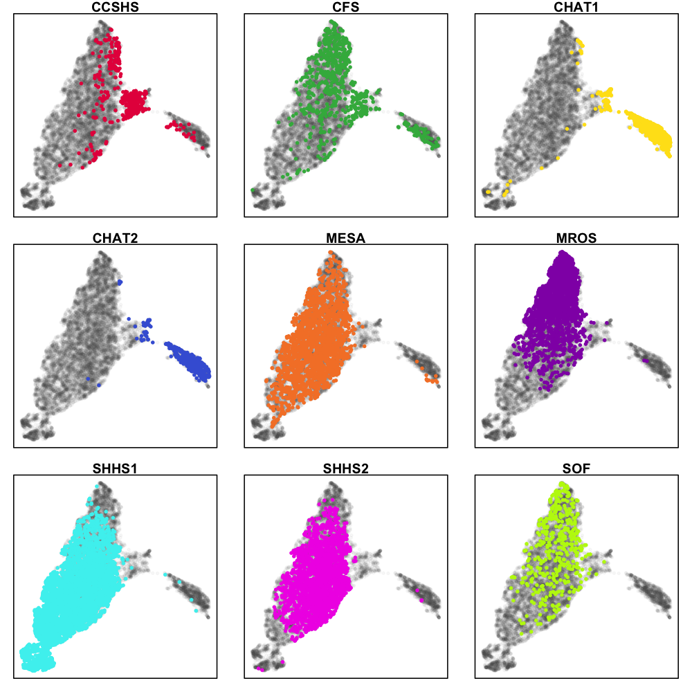
The distribution of CCSHS (16-18 year old adolescents, coloured red) is interesting, in that they largely form their own cluster, in between the children and the adults, although some CCSHS individuals appear to cluster more closely with either the children or the adults. Makes sense, I suppose. The CFS study contains a broad range of individuals, including older children as well as middle-aged adults.

Also of note, SHHS1 and MrOS seem to occupy different ends of the main cluster. This (most likely) could reflect technical differences: in fact, we should be very clear that all these types of analyses will likely represent some (possibly hard-to-determine) mixture of technical effects (between and within cohort) as well true differences in sleep macro- and micro-architecture.

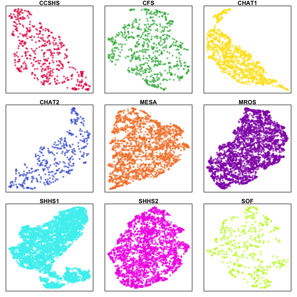
We can repeat the previous UMAP analyses, but now on one cohort at a time, i.e. to focus only on intra-cohort differences. These plots are largely uninteresting, perhaps with the exception of SHHS1, where (as evident in the early plots) there appear to be some substructure within the SHHS1 samples:

What's going on with SHHS1? Looking only at this cohort, we can flag individuals in the two lower clusters as red and blue, and then look at their power spectra (both as the mean, and also showing every individual's PSD; in all cases, the gray PSD is the mean for the rest of the SHHS1 cohort):

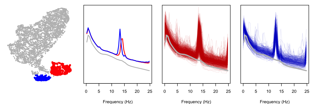
As is clear from these plots, the PSD for these subgroups contain strong spikes (at two slightly different locations, thus the appearance of more than one subgroup). Is there something terribly wrong with these studies? Not really, as a little further exploration shows, although this is also a reminder of why it is important to perform statistical artifact detection on these (and other) sleep EEGs. Based on a handful of studies selected at random, it appears that these studies contain high levels of artifact at the end of the study for the C4-M1 channel. Below, we show the power spectra for three of the "blue" individuals, along with their sleep spectrograms (i.e. epochs of sleep on the x-axis):

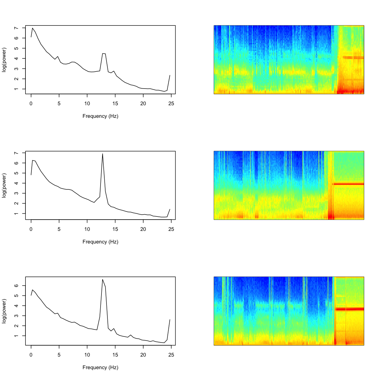
Clearly this channel has become corrupted towards the end of the recording (although these are all manually annotated as sleep epochs, meaning the other EEG channel was quite possibly still good). Note that in this analysis we purposely did not perform statistical artifact detection, as we wanted to visualize both artifactual as well as physiological sources of variation in the sleep EEG.

Clustering stages

So far, so good. But obviously we know that the sleep EEG is highly dynamic and changes with sleep stage (i.e. it is used to define sleep stage...). Averaging over all sleep epochs is not really an ideal way to consider these data, therefore. Here, we estimate the mean stage-specific PSD per individual, and use UMAP to cluster these 4N observations. That is, these plots therefore represent differences between stages as well as differences between individuals. N1, N2 and N3 are coloured light blue, blue and black; REM sleep is coloured orange. Looking at all nine NSRR cohorts together:

In the above plot, we see clear evidence of clustering both by stage and by cohort (largely CHAT versus non-CHAT), as expected. Plotting the same data separately for each of the nine cohorts:

Aside from the CHAT studies, perhaps the other noteworthy point here is that SHHS1 clustering with respect to manually-assigned stage doesn't appear as clear as for some of the other comparable cohorts (most obviously SHHS2). Although to some extent this could be a visual artifact arising from plotting twice the number of observations in one plot (SHHS1 is by far the largest study), it's still a bit curious.

Clustering epochs

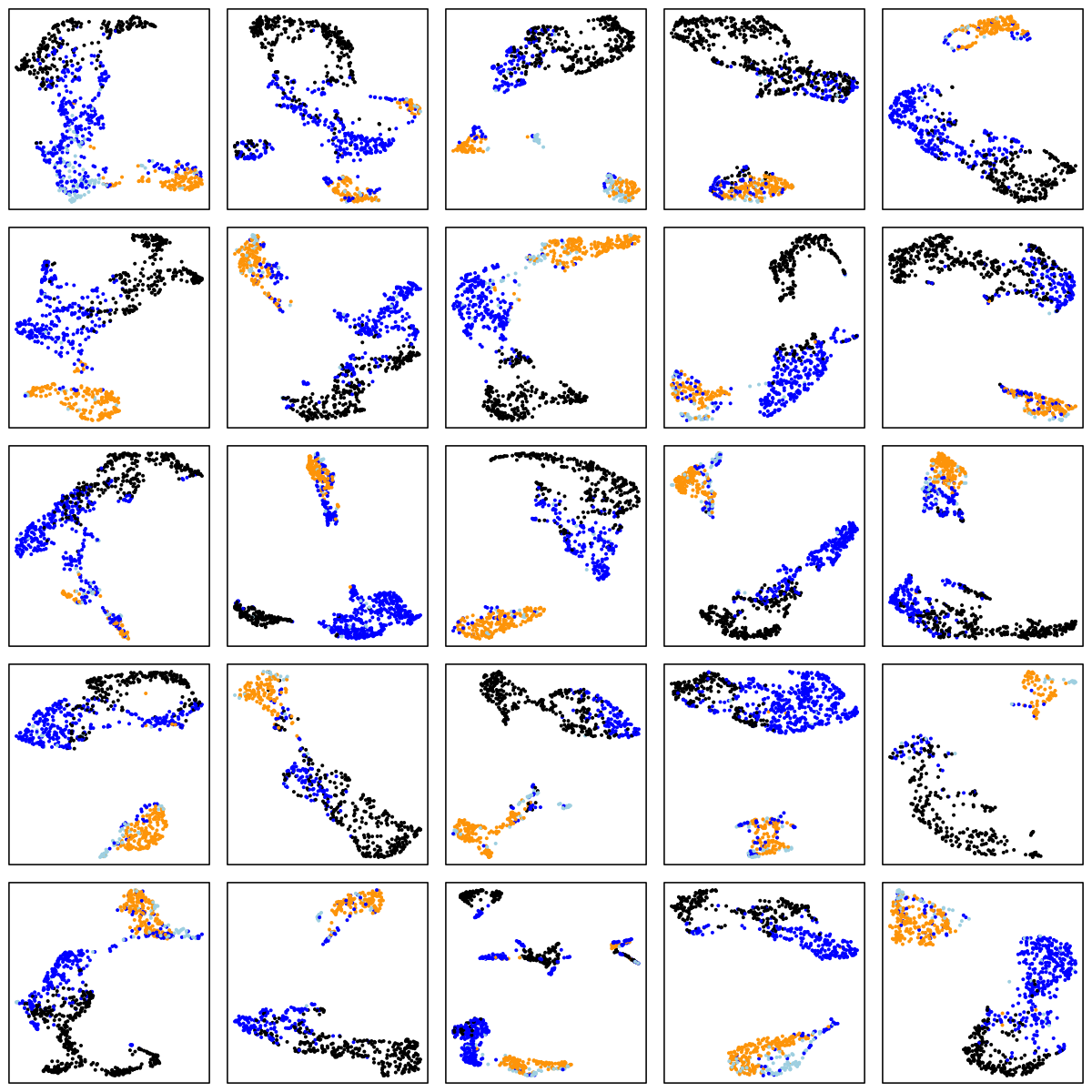
Finally, we'll use UMAP to cluster on an epoch-by-epoch basis, here within single individuals randomly selected from some of the above cohorts: CHAT (children), CCSHS (adolescents), MrOS (older adult males) and SOF (elderly females). In each case we show the results of a within-individual UMAP analysis, for 25 randomly selected individuals. As before, N1, N2 and N3 are light blue, blue and black respectively, and REM is orange:

CHAT (children)

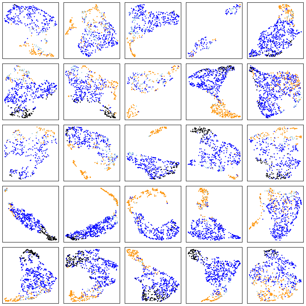
CCSHS (adolescents)

MrOS (older adult males)

SOF (elderly females)

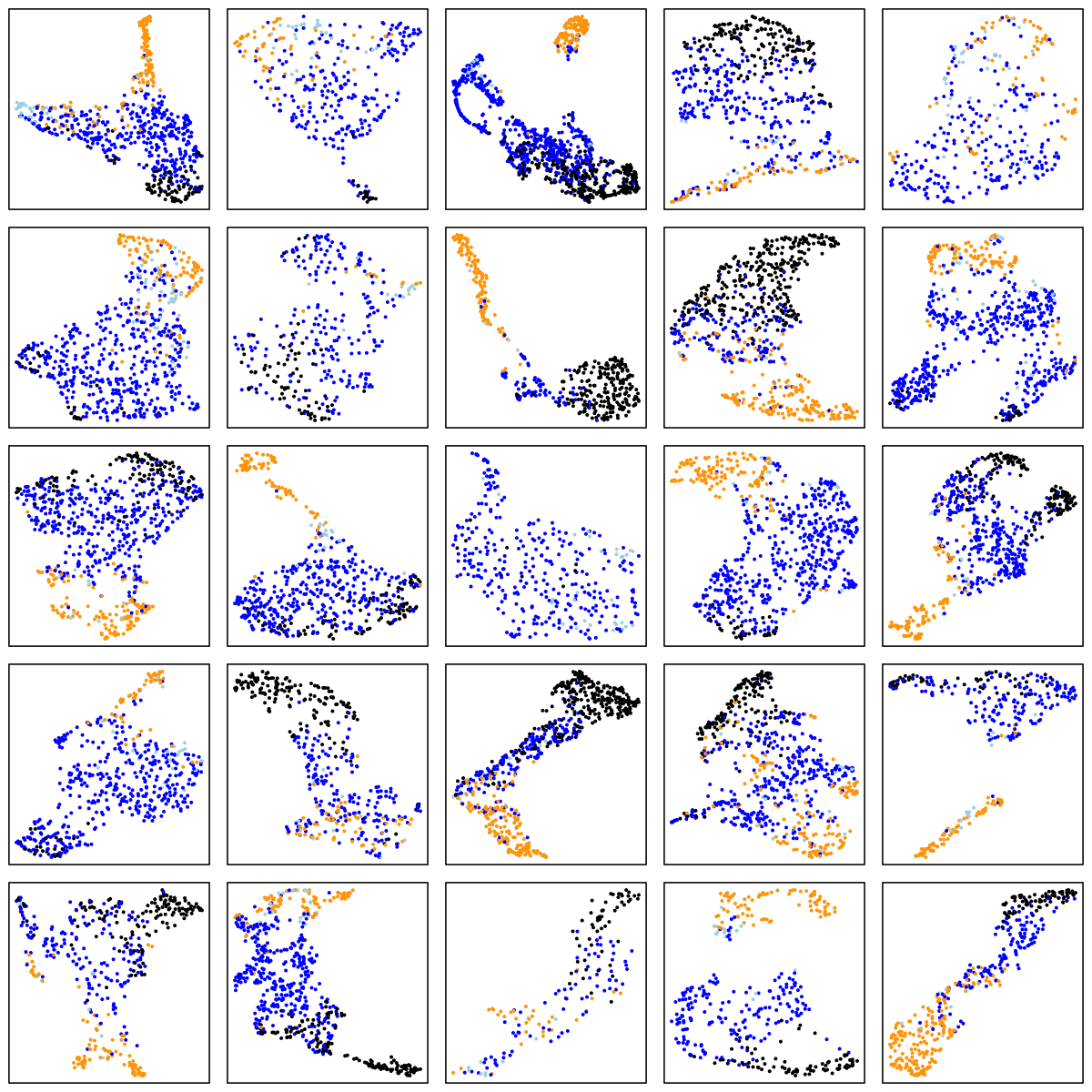
There are a number of things to note in the above plots. Perhaps most obviously is the impact of ageing on the sleep EEG: as well as fewer data-points in the two older cohorts (i.e. less sleep!), there is far less structure and separation between manually-assigned stages, and even ignoring the manual stage (as the actual UMAP analysis does), there is less evidence of substructure in each individual's sleep.

Looking at the CHAT and CCSHS plots (noting this is a very unscientific random selection of 25 individuals only from each cohort), it is interesting to note that some individuals appear to have a clear separation between N2 and N3 epochs, whereas others do not. In these latter cases, N2 and N3 epochs are often not completely overlapping, but it appears as if there is a continuum of intermediate states (which effectively acts to "join" the two stages), rather than these states being completely distinct. Often REM sleep clusters very obviously apart from N2 and N3 sleep, although of course note that (on the basis of a single EEG), REM sleep will often be not easy to distinguish between N1 and wake (we removed all wake epochs prior to the UMAP analyses).

There are also cases where artifact perhaps, or changes in the recording parameters throughout the night, seems to create substructure in these epoch-level plots. Finally, at least on the basis of this one EEG channel there appear to be a modest but non-negligible number of instances whether the manually assigned stages do not seem to agree with the data-driven patterns of clustering we see in the sleep EEG.

Conclusion

As per our stated intention, we used UMAP to visualize some NSRR data. Aside from generating some nice images summarizing approximately two months worth of sleep EEG, we haven't necessarily learned that much new. But hopefully it gives some appreciation of how artifactual and genuine sources of variation come together in "big data" analyses, and that you should always take care to tease them apart.

But perhaps the most obvious take-away: if you're developing an automated staging algorithm, it will make your performance look much better if you train and test in young samples ;-)