Maximum Likelihood Estimation (MLE)

MLE in Practice
Analytic MLE
Sometimes we can write a simple equation that describes the
likelihood surface (e.g. the line we plotted in the coin
tossing example) that can be differentiated.
In this case, we can find the maximum of this curve by
setting the first derivative to zero. That is, this represents
the peak of a curve, where the gradient of the curve turns from being
positive to negative (going left to right). In theory, this will
represent the maximum likelihood estimate of the parameter.
Numerical MLE
But often we cannot, or choose not, to write an equation that
can be differentiated to find the MLE parameter estimates. This
is especially likely if the model is complex and involves many
parameters and/or complex probability functions (e.g. the normal
probability distribution).
In this scenario, it is also typically not feasible to evaluate
the likelihood at all points, or even a reasonable number of points,
in the parameter space of the problem as we did in the
coin toss example. In that example, the parameter space was
only one-dimensional (i.e. only one parameter) and ranged
between 0 and 1. Nonetheless, because p can theoretically
take any value between 0 and 1, the MLE will always be an approximation
(albeit an incredibly accurate one) if we just evaluate the likelihood
for a finite number of parameter values. For example, we chose to
evaluate the likelihood at steps of 0.02. But we could have chosen
steps of 0.01, of 0.001, of 0.000000001, etc. In theory and practice,
one has to set a minimum tolerance by which you are happy for your
estimates to be out. This is why computers are essential for these
types of problems: they can tabulate lots and lots of values very
quickly and therefore achieve a much finer resolution.
If the model has more than one parameter, the parameter space will grow
very quickly indeed. Evaluating the likelihood exhaustively becomes
virtually impossible - even for computers. This is why so-called
optimisation (or minimisation) algorithms have
become indispensable to statisticians and quantitative scientists in the
last couple of decades. Simply put, the job of an optimisation algorithm
is to quickly find the set of parameter values that make the
observed data most likely. They can be thought of as intelligently
playing some kind of hotter-colder game, looking for a hidden object,
rather than just starting at one corner and exhaustively searching the room.
The 'hotter-colder' information these algorithms utilise essentially comes
from the way in which the likelihood changes as the they move
across the parameter space. Note that it is precisely this type of 'rate
of change' information that the analytic MLE methods use - differentiation
is concerned with the rate of change of a quantity (i.e. the
likelihood) with respect to some other factors (i.e. the parameters).
Other Practical Considerations
Briefly, we shall look at a couple of shortcuts and a couple of
problems that crop up in maximum likelihood estimation using
numerical methods:
Removing the constant
Recall the likelihood function for the binomial distribution:
 In the context of MLE, we noted that the values representing the data
will be fixed: these are n and h. In this case, the
binomial 'co-efficient' depends only upon these constants.
Because it does not depend on the value of the parameter p
we can essentially ignore this first term. This is because any value
for p which maximises the above quantity will also maximise
 This means that the likelihood will have no meaningful scale in and of
itself. This is not usually important, however, for as we shall see,
we are generally interested not in the absolute value of the likelihood
but rather in the ratio between two likelihoods - in the
context of a likelihood ratio test.
We may often want to ignore the parts of the likelihood that do not
depend upon the parameters in order to reduce the computational
intensity of some problems. Even in the simple case of a binomial
distribution, if the number of trials becomes very large, the
calculation of the factorials can become infeasible (most pocket
calculators can not represent numbers larger than about 60!). (Note: in
reality, we would quite probably use an approximation of the binomial
distribution, using the normal distribution that does not involve the
calculation of factorials).
Log-likelihood
Another technique to make life a little easier is to work with
the natural log of likelihoods rather than the likelihoods themselves.
The main reason for this is, again, computational rather than theoretical.
If you multiply lots of very small numbers together (say all less than
0.0001) then you will very quickly end up with a number that is too small
to be represented by any calculator or computer as different from zero.
This situation will often occur in calculating likelihoods, when we are
often multiplying the probabilities of lots of rare but independent events
together to calculate the joint probability.
With log-likelihoods, we simply add them together rather than multiply
them (log-likelihoods will always be negative, and will just get larger
(more negative) rather than approaching 0). Note that if
a = bc
then
log(a) = log(b) + log(c)
So, log-likelihoods are conceptually no different to normal likelihoods.
When we optimise the log-likelihood (note: technically, we will be
minimising the negative log-likelihood) with respect to
the model parameters, we also optimise the likelihood with respect to
the same parameters, for there is a one-to-one (monotonic) relationship
between numbers and their logs.
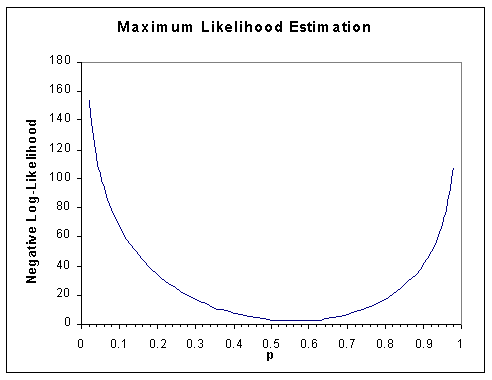
For the coin toss example above, we can also plot the log-likelihood.
We can see that it gives a similar MLE for p (note: here we
plot the negative of the log-likelihood, merely because most optimisation
procedures tend to be formulated in terms of minimisation rather than
maximisation).
 Model identification
It is worth noting that it is not always possible to find one set
of parameter values that uniquely optimises the log-likelihood. This
may occur if there are too many parameters being estimated for the
type of data that has been collected. Such a model is said to be
'under-identified'.
A model that attempted to estimate additive
genetic variation, dominance genetic variation and the
shared environmental component of variance from just MZ and DZ twin
data would be under-identified.
Local Minima
Another common practical problem when implementing model-fitting
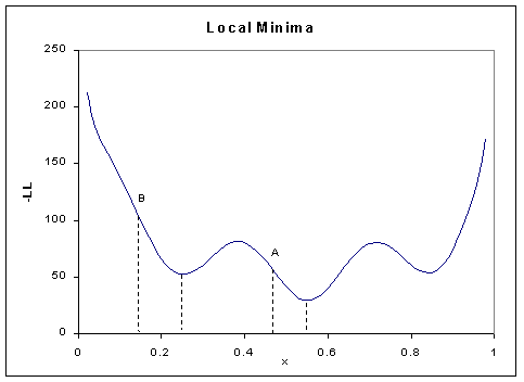
procedures is that of local minima. Take the following graph, which
represents the negative log-likelihood plotted by a parameter value,
x.
 Model fitting is an iterative procedure: the user has to
specify a set of starting values for the parameters
(essentially an initial 'first guess') which the optimisation
algorithm will take and try to improve on.
It is possible for the 'likelihood surface' to be any complex
function of a parameter value, depending on the type of model and the
data. In the case below, if the starting value for parameter x
was at point A then optimisation might find the true,
global minimum. However, if the starting value was at point
B then it might not find instead only a local minimum. One
can think of the algorithm crawling down the slope from B
and thinking it has reached the lowest point when it starts to
rise again. The implication of this would be that the optimisation
algorithm would stop too early and return a sub-optimal estimate
of the parameter x. Avoiding this kind of problem often
involves specifying models well, choosing appropriate optimisation
algorithms, choosing sensible starting values and more than a modicum
of patience.

Return to front page
Site created by S.Purcell, last updated 21.09.2000
|


