Behavioural Genetic Interactive Modules
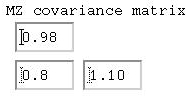
Model-fitting to Twin Data : 2 OverviewThis on-line module provides an easy way to explore the properties of the univariate ACE twin model. The user inputs the twin covariance matrices, the sample sizes and the level of significance used to compare models. The module returns the maximum-likelihood estimates for the ACE and nested submodels, determines the best-fitting model and gives standardised estimates of the model parameters for the best-fitting model.TutorialBegin by entering the observed MZ and DZ covariance matrices into the forms. In the first example, all the MZ and DZ variances are 1. This is equivalent to modeling correlations rather than covariances, and will give slightly biased results in terms of model-fit. For the purpose of this module, we shall ignore this for now. For model-fitting to work well (or work at all) the covariance matrices must conform to the basic assumptions and requirements of the model:
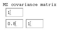
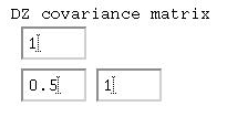 Given that the 'variances' are all 1, we can say that the
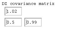
correlation between MZ twins is 0.80, whilst between
DZ twins it is 0.50. Remembering the basic formula for
calculating the heritability of a measure from the
twin correlations (i.e. twice the difference) we can
conclude that the trait is 2*(0.80-0.50) = 0.60, 60%
percent heritability.
Let's see how model-fitting compares with this estimate.
Given that the 'variances' are all 1, we can say that the
correlation between MZ twins is 0.80, whilst between
DZ twins it is 0.50. Remembering the basic formula for
calculating the heritability of a measure from the
twin correlations (i.e. twice the difference) we can
conclude that the trait is 2*(0.80-0.50) = 0.60, 60%
percent heritability.
Let's see how model-fitting compares with this estimate.
When all of these pieces of information are entered, click the
 button can be used to clear the values entered into
the webpage.
button can be used to clear the values entered into
the webpage.
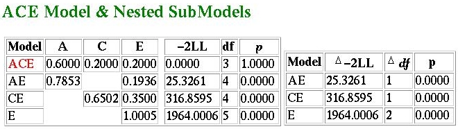
The ResultsThe results for this particular analysis are given below: they are formatted in a way similar to how many model-fitting analyses might be reported in journals: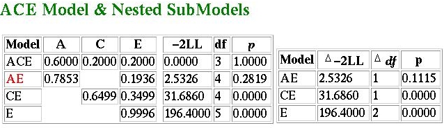 So, what do they tell us? The best-fitting model is highlighted
in red - here we see that the AE model seems to provide the
most parsimonious explanation of the observed data. But wasn't
the heritability 60%, as we calculated by taking the difference
between MZ and DZ correlations? Not under the AE model...
This represents the difference between model-fitting approaches
and the more basic approach. In this case, for these particular
data, the ACE model does produce best-fitting parameter estimates
that concur with the correlation method. That is, the A
parameter is 0.60 (representing a heritability of 60% as the
total variance, A+C+E is 1). Likewise, E is estimated at
0.20 (which corresponds to 1 minus the MZ correlation in
this case).
When comparing the difference in fit between the ACE and the
AE model, however, the model-fitting method has determined
that, given the user-specified criterion for significance, which
was 0.05 in this case, the AE model does not represent a
significantly worse explanation of the observed data. The
model fit is in the column label -2LL. This stands for
minus twice the log-likelihood, but just think of the numbers in
this column as chi-squared statistics (with the degrees of
freedom given in the df column to the right).
The fit for the ACE model is 0: a perfect fit. This is because
the model is saturated as a consequence of the variances
all being equal. The fit-function for the AE model is only 2.5326,
however. This has an associated p-value of 0.2819,
which suggests that, in absolute terms, the data do not depart
significantly from the expected predictions of the model.
Looking at the smaller table to the right gives the model
comparison tests: to ask whether the AE model provides a
better fit to the data than the ACE we test the difference
in fit-function against the difference in degrees of freedom.
In this case, as 2.5326 - 0 = 2.5326 with 4-3 = 1 degrees
of freedom is not significant at the 5% level (p=0.1115)
we can conclude that the AE provides a no-worse fit to the
data.
This is not the case with the CE model or the E model, however.
In both cases we see that they lead to a significant reduction in
fit when compared against the ACE model.
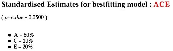
The standardised estimates for the best fitting model are given
below:
So, what do they tell us? The best-fitting model is highlighted
in red - here we see that the AE model seems to provide the
most parsimonious explanation of the observed data. But wasn't
the heritability 60%, as we calculated by taking the difference
between MZ and DZ correlations? Not under the AE model...
This represents the difference between model-fitting approaches
and the more basic approach. In this case, for these particular
data, the ACE model does produce best-fitting parameter estimates
that concur with the correlation method. That is, the A
parameter is 0.60 (representing a heritability of 60% as the
total variance, A+C+E is 1). Likewise, E is estimated at
0.20 (which corresponds to 1 minus the MZ correlation in
this case).
When comparing the difference in fit between the ACE and the
AE model, however, the model-fitting method has determined
that, given the user-specified criterion for significance, which
was 0.05 in this case, the AE model does not represent a
significantly worse explanation of the observed data. The
model fit is in the column label -2LL. This stands for
minus twice the log-likelihood, but just think of the numbers in
this column as chi-squared statistics (with the degrees of
freedom given in the df column to the right).
The fit for the ACE model is 0: a perfect fit. This is because
the model is saturated as a consequence of the variances
all being equal. The fit-function for the AE model is only 2.5326,
however. This has an associated p-value of 0.2819,
which suggests that, in absolute terms, the data do not depart
significantly from the expected predictions of the model.
Looking at the smaller table to the right gives the model
comparison tests: to ask whether the AE model provides a
better fit to the data than the ACE we test the difference
in fit-function against the difference in degrees of freedom.
In this case, as 2.5326 - 0 = 2.5326 with 4-3 = 1 degrees
of freedom is not significant at the 5% level (p=0.1115)
we can conclude that the AE provides a no-worse fit to the
data.
This is not the case with the CE model or the E model, however.
In both cases we see that they lead to a significant reduction in
fit when compared against the ACE model.
The standardised estimates for the best fitting model are given
below:
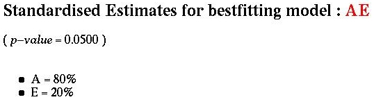 Given that the total variance was 1, these simply represent
rounded versions of the parameter estimates.
Given that the total variance was 1, these simply represent
rounded versions of the parameter estimates.
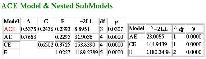
 In short, no! What we see here is that the ACE model is
selected as the best-fitting model. The parameter values
have not changed though (slight changes
might occur due to the nature of optimisation).
So why has the best-fitting model changed? The AE model
now represents a significantly worse description of the
data compared to the ACE model - this can be seen in the
comparison of fit-functions. The increased sample
size has directly lead to an increase in these functions
(note that the chi-squared values are ten times greater -
i.e. the same increase as in sample size). A chi-squared
of 25.326 with one degree of freedom is significant,
whereas 2.5326 is not.
Should this worry us? Were the answers 'wrong' before? No,
it should not worry us unduly and it does not mean that
the answers were wrong before. The difference in result
represents the fact that, with the larger sample, there
is essentially much more weight placed upon the exact
values of the observed statistics. That is, because of
the nature of random sampling, they are much less likely
to be wrong (or, more to the point, the true values are
likely to be much closer to the observed values than with
a smaller sample). If you tossed a coin 5 times and got
3 heads, you wouldn't call it biased. If you tossed a
coin 500 times and got 300 heads, you probably would
(statistically speaking, you certainly should). In
this case, the larger sample results in us not
being able to deny the existence of a shared
environmental effect amongst twins.
The standardised estimates now concur with the
estimate based on twin correlations:
In short, no! What we see here is that the ACE model is
selected as the best-fitting model. The parameter values
have not changed though (slight changes
might occur due to the nature of optimisation).
So why has the best-fitting model changed? The AE model
now represents a significantly worse description of the
data compared to the ACE model - this can be seen in the
comparison of fit-functions. The increased sample
size has directly lead to an increase in these functions
(note that the chi-squared values are ten times greater -
i.e. the same increase as in sample size). A chi-squared
of 25.326 with one degree of freedom is significant,
whereas 2.5326 is not.
Should this worry us? Were the answers 'wrong' before? No,
it should not worry us unduly and it does not mean that
the answers were wrong before. The difference in result
represents the fact that, with the larger sample, there
is essentially much more weight placed upon the exact
values of the observed statistics. That is, because of
the nature of random sampling, they are much less likely
to be wrong (or, more to the point, the true values are
likely to be much closer to the observed values than with
a smaller sample). If you tossed a coin 5 times and got
3 heads, you wouldn't call it biased. If you tossed a
coin 500 times and got 300 heads, you probably would
(statistically speaking, you certainly should). In
this case, the larger sample results in us not
being able to deny the existence of a shared
environmental effect amongst twins.
The standardised estimates now concur with the
estimate based on twin correlations:
The reason for this is that the correlation method implicitly assumes all four variances to be equal (because they have been standardised). In the previous examples, the variances were in fact all equal (the fact they were all also equal to 1 was irrelevant here). Of course, in real life all four variances could turn out to be equal, but usually they will not be identical. They should be similar, but not identical. Let's consider a situation such as this:
How does this impact on the model-fitting?
We see here that the ACE model no longer has a fit-function of zero: that is, it can no longer provide a perfect description of the data. The fit-function is 8.8951, which has a p-value of 0.0307 for three degrees of freedom. This implies that even the predictions of the ACE model significantly depart from what we have observed. As we saw in the previous tutorial, the ACE model predicts equality of variance: if this is sufficiently violated, the model will not fit. Given that, for this particular example, the sample size is quite large (1000 pairs of each zygosity) it is telling us that we have observed greater fluctuation in variance than we should expect by chance. This might indicate to the researcher to look more carefully into what is going on in the sample.
Questions
Answers
Please refer to the Appendix for further discussion of model-fitting. Site created by S.Purcell, last updated 6.11.2000 |
 Finally, we have to let the module know what significance
level to use when deciding whether or not to reject a model
in favour of a slightly worse-fitting but more parsimonious
model. It is called the User-defined type I error rate
in this module - it is otherwise known as the critical value,
the significance level, or sometimes just alpha.
This represents the probability of wrongly rejecting a model
(i.e. 5% in this case).
Finally, we have to let the module know what significance
level to use when deciding whether or not to reject a model
in favour of a slightly worse-fitting but more parsimonious
model. It is called the User-defined type I error rate
in this module - it is otherwise known as the critical value,
the significance level, or sometimes just alpha.
This represents the probability of wrongly rejecting a model
(i.e. 5% in this case).
 button to start the analysis.
You will get an error if any of these items are missing or
have invalid values (e.g. negative sample size). At the
moment the module does not capture these errors, so please
be careful with what you enter!
button to start the analysis.
You will get an error if any of these items are missing or
have invalid values (e.g. negative sample size). At the
moment the module does not capture these errors, so please
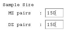
be careful with what you enter! 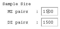 What if our sample had been larger, though? Say we observed ten
times the number of twin pairs we had previously, but that we
also observed exactly the same pattern of variances
and covariances. Does model-fitting give the same results?
What if our sample had been larger, though? Say we observed ten
times the number of twin pairs we had previously, but that we
also observed exactly the same pattern of variances
and covariances. Does model-fitting give the same results?
 Say we observed the following MZ and DZ covariance
matrices for 1000 MZ pairs and 1000 DZ pairs.
Although these data are similar to the previous
examples, the four variances vary themselves.
Say we observed the following MZ and DZ covariance
matrices for 1000 MZ pairs and 1000 DZ pairs.
Although these data are similar to the previous
examples, the four variances vary themselves.