Behavioural Genetic Interactive Modules
Covariance

Overview
Covariance is a fundamental statistic that informs us about the
relationship between two characteristics (such as height and weight,
for example). This module aims to show how this measure of association
is calculated, and how it is related to the concept of variance.
Tutorial
This module, covariance.exe is very similar to the previous
module that illustrated the calculation of variance. This is
unsurprising, for statistically and conceptually covariance is indeed
very similar to variance - that is, it is a measure of co-variation
between two traits.
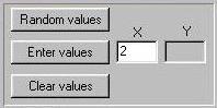 This first panel controls the input of data into the module,
and is similar to that of the variance module except that we
are now dealing with pairs of scores rather than individual
scores. Each observation represents, say, one individual and
the pair of scores represents two measures for each individual,
X and Y. The module will calculate the
covariance between X and Y.
This first panel controls the input of data into the module,
and is similar to that of the variance module except that we
are now dealing with pairs of scores rather than individual
scores. Each observation represents, say, one individual and
the pair of scores represents two measures for each individual,
X and Y. The module will calculate the
covariance between X and Y.
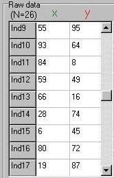 As before, the module tabulates scores, this time in pairs. In this
case, for example, the 15th individual in the sample has
scored 6 on measure X and 45 on measure Y.
As before, the module tabulates scores, this time in pairs. In this
case, for example, the 15th individual in the sample has
scored 6 on measure X and 45 on measure Y.
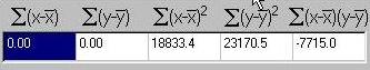
 The univariate statistics such as the sum and mean for
X and Y are calculated and displayed as before. In this case we
see, for example, that measure X has a sum of 1374 and a mean of
52.85 in the sample of the 26 individuals entered into the module.
The univariate statistics such as the sum and mean for
X and Y are calculated and displayed as before. In this case we
see, for example, that measure X has a sum of 1374 and a mean of
52.85 in the sample of the 26 individuals entered into the module.
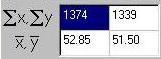
 For bivariate data, as well as plotting a bar
chart for each measure, we can also plot a
scatter-plot that gives a visual representation
of the association between the two measures. Each point
represents an individual, the horizontal axis represents
their score on X, the vertical axis their score on Y. The
little lines plotted on the axes represent 1 and 2
standard deviations away from the mean.
For bivariate data, as well as plotting a bar
chart for each measure, we can also plot a
scatter-plot that gives a visual representation
of the association between the two measures. Each point
represents an individual, the horizontal axis represents
their score on X, the vertical axis their score on Y. The
little lines plotted on the axes represent 1 and 2
standard deviations away from the mean.
From the scatter-plot, we can see that the two variables do not
seem to be strongly related. If anything, there appears
to be a slight negative association, in that
individuals who score higher on X seem to, on average,
score slightly lower on Y. The covariance statistic we
are about to calculate will quantify this relationship
more precisely.
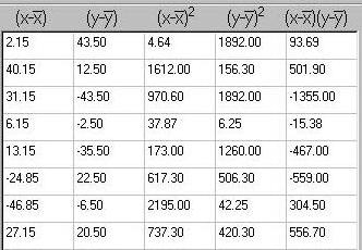 For both X and Y we calculate the deviations from the
mean, and square these deviations. These are used in the
calculation of variance. The fifth column represents
the quantity that is most relevant to covariance however:
the cross-product of the deviation from the mean
for X and the deviation from the mean for Y for each
individual. For example, in the top line here we see that
this individual has scored 2.15 units above the mean on X
and 43.5 units above the mean on Y. The cross-product is
simply 2.15 multiplied by 43.5, or 93.69.
For both X and Y we calculate the deviations from the
mean, and square these deviations. These are used in the
calculation of variance. The fifth column represents
the quantity that is most relevant to covariance however:
the cross-product of the deviation from the mean
for X and the deviation from the mean for Y for each
individual. For example, in the top line here we see that
this individual has scored 2.15 units above the mean on X
and 43.5 units above the mean on Y. The cross-product is
simply 2.15 multiplied by 43.5, or 93.69.
Note how some of these cross-products are negative,
unlike the squared deviations from the mean. This
represents the fact that covariance represents not just
a measure of strength of association, but also implies a
direction of association. In this context, negative
values reflect scoring higher than average on one
measure but lower than average on the other measure.
In a similar manner, these squared deviations are summed,
as are the cross-products. Note how, in this instance, the
sum of cross-products is actually negative.
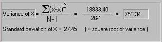 For both X and Y we can use the sum of squared deviations
from the mean to calculate the variance of each measure,
as in the previous module. This picture shows the variance
calculated for X.
For both X and Y we can use the sum of squared deviations
from the mean to calculate the variance of each measure,
as in the previous module. This picture shows the variance
calculated for X.
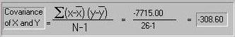 Here we calculate the covariance: whereas the variance of
one measure is the average squared deviation from the mean,
the covariance between two measures is the average cross-product
of deviations from the mean for the two measures. In this case,
the covariance is -308.6, confirming the impression given
by the scatter-plot that X and Y appear to be negatively
associated.
Here we calculate the covariance: whereas the variance of
one measure is the average squared deviation from the mean,
the covariance between two measures is the average cross-product
of deviations from the mean for the two measures. In this case,
the covariance is -308.6, confirming the impression given
by the scatter-plot that X and Y appear to be negatively
associated.
So what does -308.6 mean? Is this a strong negative
association? Is this meaningfully different from a covariance
of zero, implying no association? As you might expect, in
order to answer such questions, we have to take into
consideration the individual variances of each measure.
That is, if the variances of X and Y were both around
10,000 then the absolute magnitude of the covariance, only
in the hundreds, would mean that the covariation between X
and Y was relatively small compared to the variation in
the measures that was not shared between them. If
the variances were of the order of four or five hundred,
however, then the majority of the variance would appear to
be shared. This kind of calculation is precisely what a
correlation does: the correlation
coefficient will be introduced in the next module.
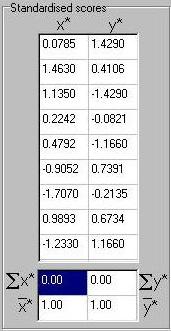 Finally, the standardised scores for both X and Y
are given: these are calculated in an identical manner
to the variance module.
[note: correct error on labels of
screen-shot]
Finally, the standardised scores for both X and Y
are given: these are calculated in an identical manner
to the variance module.
[note: correct error on labels of
screen-shot]
Questions
- If X and Y are two variables with the same variance, would it
ever be possible for the covariance between
X and Y to be greater than their variances? If not, why not?
- Use the module to calculate the covariance
between the two measures in the following
sets. What do the covariances tell you about
the relationship between the two variables here?
- X : 1, 2, 3, 4, 5, 6, 7
Y : 2, 3, 4, 5, 6, 7, 8
- X : 1, 2, 3, 4, 5, 6, 7
Y : 2, 4, 6, 8, 10, 12, 14
- X : 60, 55, 45, 60, 45
Y : 60, 55, 65, 50, 45
- X : 5, 5, 5, 5, 5, 5, 5
Y : 1, 2, 3, 4, 5, 6, 7
- Would it tell you anything if you were to
recalculate a covariance on standardised
scores instead of raw scores?
Answers
- In short, no. If you think of a covariance as a
measure of association, it is obvious that a trait
is completely 'associated' with itself.
If two measures had the same
variance, it would be possible for the covariance to
equal the variance. The only way this
could happen if the two variables have identical
deviations from the mean for every single observation,
however. Two such variables could not really be considered
to measure different things in any case.
- The first set of numbers represent the case we
mentioned above, where the covariance is equal
to the two variances. That is, there is a perfect
linear association between X and Y, even though
Y has a greater mean than X.
The contrast with the first set of numbers is
interesting here. There is also a perfect linear relationship
between X and Y. In this case, X and Y have different variances,
however, so the covariance is different from above.
In the third set, X and Y are unrelated. That is, the covariance
is zero. Note how the cross-products of the deviations from
the mean cancel themselves out, so that the sum is 0.
In the final set, we see that X has a variance of 0, as
there is simply no variation in the scores: they are all 5.
The covariance is necessarily 0 also: if a trait doesn't vary,
it cannot covary with any other trait.
- Yes it would: in fact, this is the basis of the
correlation coefficient, which we shall review in
the next module. As an exercise now, re-enter the values for
the first two sets of numbers from the last question. Make
a note of the pairs of standardised scores for both sets.
Then try entering the standardised scores into the module
as input in both cases.
You will find that the standardised scores are the
same for both cases; when entered the variance of both
X and Y will be 1, in both cases, because they have
been standardised. The covariance will be 1 in both
cases also. This actually represents the correlation
between X and Y, as we shall see in the next module.
The fact that this quantity is now the same for the
first and second sets of numbers represents the
'standardised' nature of the correlation: in both
cases the association between X and Y is equally
strong, all that changes is the scale (variance) of
one of the measures.
Please refer to the Appendix for further discussion of
what covariances represent and how they are used.
Site created by S.Purcell, last updated 12.11.2000
|