Behavioural Genetic Interactive Modules

Matrices

Overview

This module aims to familiarise individuals with some of the common operations in matrix algebra.

Tutorial

This module allows the user to perform some of the more common matrix operations, such as matrix addition, multiplication, inversion and transposition. Some of these functions operate on only one matrix, such as inversion, whereas some take two matrices to produce a resulting matrix, such as addition. Also, certain operations require the matrix or matrices to have certain properties, such as being square, of having nonzero diagonal elements.

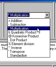Firstly, select the type of matrix operation you wish to perform: use the pull-down menu in the top-middle of the screen. For example, we choose to multiply two matrices together in this instance. As matrix multiplication is a function that takes two matrices to produce a resulting product matrix, both matrices A and B remain on screen. Matrix B will disappear if a function is selected that requires only one matrix (these are called unary functions, as opposed to binary functions).

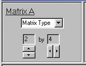We can define the sizes of matrices A and B using the arrows in the Matrix A and Matrix B panels. The maximum number of rows and columns is four. Also, certain predefined types of matrix can be selected from the pull-down menu in each panel. [Not operational yet]

The different types of matrix are described below :

Full

Every element can be any value. For example, here is a full 2-by-2 matrix:

23	12
56	16

Lower Triangular

Only the elements on the diagonal and below are represented (the others are assumed to be zero). Such a representation is commonly used to symmetric matrices also (the other elements are assumed to be identical to the below-diagonal elements). Here is a 3-by-3 lower triangular matrix:

0.23
0.12	0.52
0.76	0.14	0.73

Diagonal

All off-diagonal elements are zero:

(x+2d)	0	0
0	y²	0
0	0	4z

Zero

All elements are zero:

0	0
0	0

Unit

All elements are one:

1	1
1	1

Identity

All diagonal elements are 1, all off-diagonal elements are zero.

1	0	0
0	1	0
0	0	1

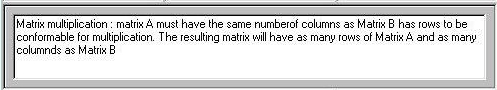Upon selecting the type of function, some text will be displayed in the middle window, telling the user whether or not there are any special conditions required for that type of operation. In this case, for multiplication to be possible between two matrices (we say that they are conformable for multiplication) the first matrix must have the same number of columns as the second matrix has rows.

Different functions have different requirements:

Addition: Both matrices must be exactly the same size
Subtraction: Both matrices must be exactly the same size
Multiplication: Matrix A must have as many columns as Matrix B has rows
Quadratic Product: Matrix B must be square and have the same number of columns as Matrix A does
Kronecker Product: Technically no restrictions, although in this module, the resulting matrix cannot be larger than a 4-by-4 matrix
Dot Product: Both matrices must be exactly the same size
Element Division: Both matrices must be exactly the same size
Inversion (unary operation): The matrix must be square and positive-definite. For this module, we only calculate the inverse of symmetric matrices, also - the module only looks at the lower triangular elements.
Transposition (unary operation): No restrictions
Standardisation (unary operation): The matrix must be square and not have any zeros along the diagonal

Let's consider the example of matrix multiplication. We know that Matrix A must have the same number of columns as Matrix B has rows. In this case, Matrix A has 2 rows and 4 columns, whereas Matrix B has 4 rows and 2 columns. They are conformable for multiplication. The resulting matrix will have as many rows as matrix A and as many columns as matrix B. It is always common to write the number of rows before columns when talking about the dimension of a matrix. Therefore :


        Matrix A      Matrix B

	 R   C         R   C 

	 2   4         4   2 
	 |   |  equal? |   |
	 |   |---------|   |
	 |                 |
	 |-----------------|
         dimension of product

The two inner numbers must be equal, the resulting matrix has the dimension given by the two outer numbers.

In our example, we expect a 2-by-2 matrix to result, therefore. Matrix multiplication is introduced in the Appendix: remember that the basic principle is that the i^th, j^th element in the resulting matrix is the sum of the products of all the elements in the i^th row in Matrix A with the corresponding element in the j^th column of Matrix B. In this case:

30 = 1*1 + 2*2 + 3*3 + 4*4
70 = 5*1 + 6*2 + 7*3 + 8*4
70 = 1*5 + 2*6 + 3*7 + 4*8
174 = 5*5 + 6*6 + 7*7 + 8*8

Different matrix operations

Matrix multiplication seems quite different to usual multiplication. The equivalent of 'normal' multiplication is called the dot product, where the [i,j] element of matrix A is multiplied by the [i,j] element of matrix B to give the [i,j] element of the resulting matrix. [This is Mx's definition of a dot product]

Element division is similar to the dot product in this respect. The matrix equivalent of division is concerned with the operation called inversion. This is because


  I = A * A~

where I is an identity matrix, A is a symmetric, square matrix and A~ is its inverse. This is the definition of a reciprocal, that is the inverse represents, in non-matrix notation, 1/a. Try this with some real numbers using the module. That is, make up a square symmetric matrix, calculate its inverse, then multiply the matrix by its inverse. Ignoring rounding errors, the resulting matrix will always be an identity matrix.

The transpose of a matrix (X') simply turns a matrix on its side: all the rows become columns and all the columns become rows. This is often useful in matrix operations. The equivalent of 'squaring' a lower triangular is X*X'.

As covered in the Appendix, we can also standardise matrices, by dividing the [i,j] elements by the square root of the product of elements [i,i] and [j,j]. This has the effect of making all diagonal elements 1. In this case of a covariance matrix, standardisation will produce a correlation matrix, where all the off diagonal elements are less then 1.

The quadratic product and Kronecker product are not covered in this tutorial, nor implemented in the module yet.

Questions

What other differences are there between normal multiplication and matrix multiplication? For example, is matrix A multiplied by matrix B the same as matrix B multiplied by matrix A ?

Answers

Site created by S.Purcell, last updated 6.11.2000