Behavioural Genetic Interactive Modules

Single Gene Model

Overview

When we say that a trait is heritable or genetic, we are implying that at least one gene has a measurable effect on that trait. Although most behavioral traits appear to depend on many genes, it is still important to review the properties of a single gene because the more complex models are built upon these foundations. This module aims to illustrate some facets of the basic quantitative genetic model for single genes.

Tutorial

The Appendix introduces many of the terms that are used in this module: it is recommended that you read it before reading this tutorial and using the module.

Despite being called a single gene model, this module actually allows the user to examine the effects of two genes against a background of residual variation in a population of 1000 individuals. Let's take a quick tour to familarise ourselves with the different elements of the module before we begin using it.

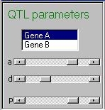This panel allows the user to control the properties of the two genes. Clicking on either Gene A or Gene B will set the three sliders to the current values for that gene. The three sliders represent the additive genetic value (a), the dominance deviation (d) and the frequency (p) of the trait-increasing allele. Both genes are bialleleic- that is, they only have two alleles.

The additive genetic value can take a value between 0 and 1 in this demo. The upper limit of 1 is arbitrary - in reality it could be any value (it will depend on the units in which the trait is measured). The dominance deviation, in this module, can be between -1 and 1. Allele frequency ranges between 0 and 1.

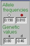These values are represented in this panel, for the selected gene only. In this case we see that Gene A has a common allele (the red allele is always the trait-increasing allele), with an additive genetic value of 0.80. In this case, heterozygotes tend to score below the homozygote midpoint (i.e below zero) due to dominance.

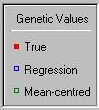
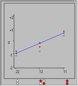The graph plots the genetic values for Gene A. As indicated by the key (illustrated right) the red dots here indicate the true genetic values. The red and white circles along the x-axis of this graph represent the three classes of genotype for this locus. The white-white genotype's genetic value is therefore plotted at -0.80 (i.e. -a). The red-white heterozygote's value is at -0.46 (i.e. d), whilst the red-red homozygote is at 0.80 (i.e. +a). The blue line represents the regression slope if we assumed only additive effects at this locus. The green points represent the mean-centred genetic values: these values take the frequency of the genotypes into account, so that the population mean will always be zero.

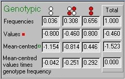These statistics are also represented in this table, along with the genotype frequencies. The bottom line illustrates the way in which the population mean is always zero based on the mean-centred genetic values.

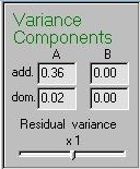We can use standard formulas to calculate the trait variance attributable to additive or dominance effects at each locus. These values are in raw score units - they are not proportions of variance. So we see that the variance attributable to the additive effects of locus A is 0.36, and 0.02 for the effects of dominance at this locus. As we have not set any values for locus B yet, these values are at zero. Normally these values would be expressed at proportions of the overall variance - e.g. that the locus accounts for, say, 4% of the variation in the trait.

The module simulates the trait scores of 1000 individuals automatically, every time one of the sliders is moved. The variation in the individuals' trait scores arise from two sources: variation due to either gene A or B, and what we call residual variation. This refers to the net effect of all the influences that operate on the trait other than these two genes. Potentially, there could be thousands of such influences. The Residual variance slider, shown in the Variance Components panel, is used to specify the variance in the trait due to factors other than the two genes. We can think of the amount of residual variation as the amount of 'noise' swamping the effects of the specific genes.

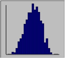When the 1000 individuals' scores are simulated, on the basis of the model specified, the module plots the distribution of trait scores as a histogram. Here we see a trait that looks more or less normally-distributed.

The slider underneath the histogram (not shown in the screenshot) is used to adjust the scale of the x-axis, so that the distribution can be clearly seen. The scale ranges from +/- 1 to +/- 10.

In this instance, the module is plotting the histogram for all 1000 individuals. By clicking on the buttons below the histogram, however, as shown here,

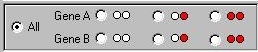the module will plot only those individuals with that certain genotype. This facilitates exploration of the effect of genes.

Using the module

Set the module to the following scenario (make sure that locus B has no effect on the trait: the easiest way to do this is to close and re-open the module). This describes a single gene with a moderately uncommon trait-increasing allele (red allele frequency is 26%) and this red allele has a reasonably large effect (a=0.80) with a slight effect of dominance (d=-0.18).

Note that, in real terms, whether or not the effect is 'large' will depend totally on the ratio of QTL variance to residual variance, of course.

[following section needs changing]

[make residual variance zero] [comment on mean centering] how pop mean always 0] [how means of the genoptyes equal the positions of the green dots] [introduce concept of QTL]
Let's make the effect large by moving the residual variance slider to the left,

to specify that the residual variance should only be 0.135 times the QTL variance. If we call the QTL variance V and the total variance T, then T = Q + (0.135*Q). The proportion of variance attributable to the QTL (i.e. Q/T) is therefore 88%, after rearranging the above equation. This would represent a major gene effect.

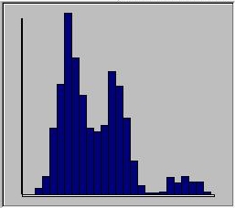Looking at the histogram, we can see this is so. The three genotypes separate quite clearly into three separate classes. The height of the peaks represent the genotype frequencies. Use the buttons to view one genotype at a time and see how they map onto this distribution. Try changing the allele frequencies and the genetic values to get a sense of how they will impact on the overall distribution of the trait.

For most quantitative, complex traits we do not observe distributions that look so discrete. There is plenty of evidence to suggest that most genes impacting on complex, quantitative traits will individually account for maybe no more than 5% of trait variation. This is equivalent to a residual variance that is 19 times greater than the QTL variance also impacting on the trait. Set the residual variance slider to as close to x19 as possible and observe how little difference in the genotypic means it is possible to observe in the histogram now.

To study the effect of two, independently acting genes, select Gene B and change the parameter values. Note how, if the residual variance is low, so that you can see clearly the different genotype classes in the histogram, you can see the pattern of genotypes of gene B if you select on gene A in the histogram and vice versa.

Site created by S.Purcell, last updated 13.11.2000