Behavioural Genetic Interactive Modules
Variance

Overview
Variance is a key concept in the measurement of individual
differences. The aim of much behavioural genetic research
is to uncover the components of variance in a
trait in order to understand what makes some individuals
differ from other individuals. This module shows how
the variance in a sample of observations is calculated
and how it can be used to standardise measurements.
Tutorial
 The Windows module, variance.exe, allows a number
of data points on a single measure to be tabulated and for
the variance calculated. Upon opening the module, you will
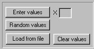
see a window with several panels. The top left panel provides three
different ways of entering data: inputing specific
numbers by clicking on Enter values, generating
random numbers, by clicking on Random values, or
loading numbers from a file, Load from file.
The following pages contain example files of well
different distributions that can be loaded into the
demonstration:
The Windows module, variance.exe, allows a number
of data points on a single measure to be tabulated and for
the variance calculated. Upon opening the module, you will
see a window with several panels. The top left panel provides three
different ways of entering data: inputing specific
numbers by clicking on Enter values, generating
random numbers, by clicking on Random values, or
loading numbers from a file, Load from file.
The following pages contain example files of well
different distributions that can be loaded into the
demonstration:
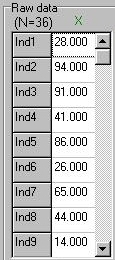 Each value entered is recorded and tabulated as seen in the screenshot
to the left. This shows 36 values have been entered (N=36), of which we
can currently see the first nine.
Each value entered is recorded and tabulated as seen in the screenshot
to the left. This shows 36 values have been entered (N=36), of which we
can currently see the first nine.
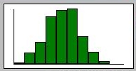
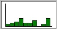 These values are automatically plotted in the form of a bar chart.
(Note that the scale of the chart is fixed from 0 to 100, so if only
very small numbers are entered, the chart will look skewed).
These values are automatically plotted in the form of a bar chart.
(Note that the scale of the chart is fixed from 0 to 100, so if only
very small numbers are entered, the chart will look skewed).
 At the bottom of the column of numbers, the sum of the
variable, X, is calculated. Dividing this by the
number of observations, N, gives the mean, which is shown
below (the X with a bar above it).
At the bottom of the column of numbers, the sum of the
variable, X, is calculated. Dividing this by the
number of observations, N, gives the mean, which is shown
below (the X with a bar above it).
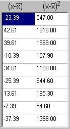 The figures to the right represent the deviations from the
mean, in the first column, and the squared deviations from
the mean. Take, for example, the first row: the data point is 28.
The mean is 51.39 for all 36 points, so the deviation from the
mean for this point is 28 - 51.39 = -23.39. And -23.39 squared is
547. This calculation is repeated for every data point.
The figures to the right represent the deviations from the
mean, in the first column, and the squared deviations from
the mean. Take, for example, the first row: the data point is 28.
The mean is 51.39 for all 36 points, so the deviation from the
mean for this point is 28 - 51.39 = -23.39. And -23.39 squared is
547. This calculation is repeated for every data point.
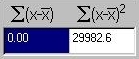 The deviations from the mean will always sum to zero (by
definition). This can be seen in the figure to the left. The
quantity of interest is the sum of the squared deviations. This
is 29982.6.
The deviations from the mean will always sum to zero (by
definition). This can be seen in the figure to the left. The
quantity of interest is the sum of the squared deviations. This
is 29982.6.
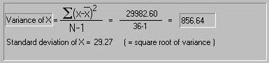 By simply taking the average of the square deviations (i.e.
dividing the sum by the number of observations) we obtain the
variance. For technical reasons, it is common practice to
subtract 1 from the number of observations in the sample (because
the same sample was also used to calculate the mean, and this
introduces a slight bias). So here we see that the variance is
29982.6 divided by 35 (36-1) which equals 856.64. The standard
deviation is simply the square root of the variance, and
is given below. Both these quantities are very useful in the
further analysis of the trait.
By simply taking the average of the square deviations (i.e.
dividing the sum by the number of observations) we obtain the
variance. For technical reasons, it is common practice to
subtract 1 from the number of observations in the sample (because
the same sample was also used to calculate the mean, and this
introduces a slight bias). So here we see that the variance is
29982.6 divided by 35 (36-1) which equals 856.64. The standard
deviation is simply the square root of the variance, and
is given below. Both these quantities are very useful in the
further analysis of the trait.
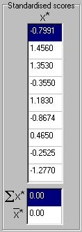 Another use of these statistics is to standardise scores.
Standard scores always have a mean of zero and a standard deviation
of 1. We can see how standard scores are calculated here: each
score is expressed as a deviation from the mean and then divided
by the standard deviation for the sample. Twenty-eight therefore is
re-expressed as -0.7991 ( (28 - 51.39) / 29.27 = -0.7991).
Another use of these statistics is to standardise scores.
Standard scores always have a mean of zero and a standard deviation
of 1. We can see how standard scores are calculated here: each
score is expressed as a deviation from the mean and then divided
by the standard deviation for the sample. Twenty-eight therefore is
re-expressed as -0.7991 ( (28 - 51.39) / 29.27 = -0.7991).
Questions
- Why will variances always be positive numbers?
- Which set of numbers have i) the greater mean, ii) the
greater variance ?
- A: 7,34,23,14,28,2,41,32,12
- B: 67, 62, 65, 66, 62, 71, 67
- C: 57, 52, 55, 56, 52, 61, 57
Answers
- Because variances are calculated from the squared
deviations from the mean, they will always be positive.
That is, the square of any number, whether positive or
negative, will always be positive itself. The average of a
set of positive numbers will also be positive itself.
- Set A has a smaller mean but a larger variance. Set
A has a mean of 21.44 but a variance of 178.53.
Set B has a mean of
65.71 but a variance of 9.9. As you might have noticed, Set
C
is similar to Set B, except each number is smaller by exactly 10.
The mean is also 10 units smaller (55.71) - but the variance is
the same (9.90). This makes sense: the variation about the
set mean is the same. That is, looking at the values entered
in the module, the deviations from the mean would have
been identical in both cases (i.e. 57 - 55.71 = 67 - 65.71).
Please refer to the Appendix for further discussion of
what variances represent and how they are used.
Site created by S.Purcell, last updated 6.11.2000
|