Behavioural Genetic Interactive Modules
 Variance Components : ACEThis module aims to illustrate the way in which variation in a quantitative trait can be attributed to different sources. Namely, we consider variation due to additive genetic effects and variation due to environmental effects, which may or may not be shared between two members of the same family.Tutorial This module is split in two halves: the first considers
variation in a sample of individuals, the second considers
variation in identical (MZ) and non-identical (DZ) twin pairs.
Clicking on the appropriate tab takes you between these
two parts (the two parts are otherwise independent
from each other).
This module is split in two halves: the first considers
variation in a sample of individuals, the second considers
variation in identical (MZ) and non-identical (DZ) twin pairs.
Clicking on the appropriate tab takes you between these
two parts (the two parts are otherwise independent
from each other).
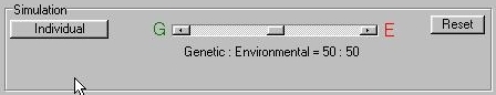 We shall begin by looking only at individuals. The module
presents a panel, shown above: clicking the Individual
button causes the module to add a new individual to the sample.
The slider on this panel represents the relative balance
of additive genetic and environmental effects for the
trait of interest. Moving the slider to the left would
indicate that genes have a stronger influence on the
trait.
When we say that genes are more important for a trait,
we mean that having a very high score or very low score
is more likely to be due to an individual's genetic makeup
rather than any environmental factors. On average, however,
the influence of genes (or environments) would neither
tend to make individuals higher nor lower.
We shall begin by looking only at individuals. The module
presents a panel, shown above: clicking the Individual
button causes the module to add a new individual to the sample.
The slider on this panel represents the relative balance
of additive genetic and environmental effects for the
trait of interest. Moving the slider to the left would
indicate that genes have a stronger influence on the
trait.
When we say that genes are more important for a trait,
we mean that having a very high score or very low score
is more likely to be due to an individual's genetic makeup
rather than any environmental factors. On average, however,
the influence of genes (or environments) would neither
tend to make individuals higher nor lower.
P = G + E
That is, a phenotype (P) is considered to result from
independent effects of genes and environment.
The two boxes shown at the bottom represent
the mean value of genetic and environmental effects. As
you add more individuals you will see that these both
tend towards zero: this would be the phenotypic population
mean of the trait also.
Changing the slider to control the relative balance will
not change the mean effect of genes or
environment in this module. Rather, if the relative
balance is heavily loaded on the genetic side, you
will see that the absolute values of the scores
is, on average, larger. That is, the effect of genes is
more likely to be very high or very low than the effect
of the environment. This is what it means to say that
'genes are more important' for the trait. Certain
constellations of genes might cause very high scores,
certain constellations might cause very low scores. In
contrast, the effects of the environment will have very
little impact on the trait, in either direction.
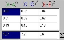
The variances for these components of the trait are calculated and shown in the panel below. The module is set such that the trait is always simulated with a mean of zero and a variance of 1 (i.e. a standardised trait). The proportions of variance will always be close to the absolute variances, therefore, but these are also shown in the panel. (Note: the sample variance will not always be exactly 1, due to the fluctuations inherent in random sampling). 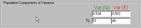 In this instance we see that the variance due to
the genetic component is approximately equal to the
variance of the environmental component, as specified
in the top panel. In this case, the relative
magnitude of these components of variance reflect
how much impact each source of variance has on the
trait and should be reflected in the pattern of
scores for the individuals in the sample.
Try changing the position of the slider to see how
this is reflected in the pattern of scores and
variances. Note that you must press the Reset
button after changing the slider, or else the
sample will represent a mixture of different populations.
The module only allows 199 individuals to be simulated.
In this instance we see that the variance due to
the genetic component is approximately equal to the
variance of the environmental component, as specified
in the top panel. In this case, the relative
magnitude of these components of variance reflect
how much impact each source of variance has on the
trait and should be reflected in the pattern of
scores for the individuals in the sample.
Try changing the position of the slider to see how
this is reflected in the pattern of scores and
variances. Note that you must press the Reset
button after changing the slider, or else the
sample will represent a mixture of different populations.
The module only allows 199 individuals to be simulated.
But...This point is very important: in reality we would never get the chance to observe the two components in this way. That is, we can only measure P. We have no direct way of knowing G or E - all we know is that they will sum to P in any one individual. We therefore have no way of directly calculating the variance of these components. This module is not meant to represent how research proceeds: this is more or less what happens in reality though. If we had measured some specific gene or some specific aspect of the environment for each individual, then we would be able to calculate the variance in the trait of interest attributable to these specific sources of variation. In this case, however, we have not measured anything else apart from the trait itself. We could not be able to say anything more about the trait over and above a simple description of the distribution of the trait in the sample. As we shall see in the second half of this module, and fundamentally, in the next module, the ability to estimate the components of variance depends crucially on basic biological theory and the measurement of the trait in related individuals. Biology predicts how similar we would expect related individuals to be because we know the expected sharing of different components of variance between different types of individuals.Twins : Shared and nonshared environmentsClicking on the Twins tab at the top of the module will bring up this slightly different panel: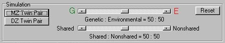 Instead of generating individuals we are now generating
pairs of twins: these twin pairs may either be monozygotic
(MZ) twins or dizygotic (DZ) twins.
The relative balance of genes and environment is still
determined in the same way by the top slider. There is
now an extra slider below, however, which represents
how much of the environmental effects are shared between
twins. Environmental effects that are shared impact
equally on both members of the twin pair. Also, this
sharing is the same for both MZ and DZ twin pairs.
In the case above, we see that the influence of genes is
just as great as the influence of the environment. The
environmental influence is then further subdivided into
a component which is shared between both members of a
twin pair and a component which is not. This latter
component we call the nonshared environment.
Therefore, the relative balance of additive genes, shared
environment and nonshared environment is 50 : 25 : 25 in
this case.
Instead of generating individuals we are now generating
pairs of twins: these twin pairs may either be monozygotic
(MZ) twins or dizygotic (DZ) twins.
The relative balance of genes and environment is still
determined in the same way by the top slider. There is
now an extra slider below, however, which represents
how much of the environmental effects are shared between
twins. Environmental effects that are shared impact
equally on both members of the twin pair. Also, this
sharing is the same for both MZ and DZ twin pairs.
In the case above, we see that the influence of genes is
just as great as the influence of the environment. The
environmental influence is then further subdivided into
a component which is shared between both members of a
twin pair and a component which is not. This latter
component we call the nonshared environment.
Therefore, the relative balance of additive genes, shared
environment and nonshared environment is 50 : 25 : 25 in
this case.
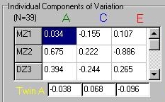 Clicking on one of the twin pair buttons causes the
module to simulate values for a twin pair, but
broken up into these three distinct components.
Again, each individual's trait score would represent
the sum of these three components. Note that there
is also a box below representing the components for
the second twin, labelled Twin B.
If an MZ twin pair is generated, note how their
scores for the additive genetic component (A) and the
shared environmental component (C) will always be
identical. The nonshared environmental effects (E) will
be different for each twin however.
For DZ twin pairs, only the shared environmental
components will be identical. The additive genetic
effects will tend to be similar, but not identical.
That is, if Twin A has a very large, positive additive
genetic effect, then it is likely that Twin B will
also have an additive genetic effect that is above
the mean (i.e. greater than zero). This will not
be the case for the nonshared effects however,
they will be unrelated between the two twins (this
will also hold for MZ twins).
Clicking on one of the twin pair buttons causes the
module to simulate values for a twin pair, but
broken up into these three distinct components.
Again, each individual's trait score would represent
the sum of these three components. Note that there
is also a box below representing the components for
the second twin, labelled Twin B.
If an MZ twin pair is generated, note how their
scores for the additive genetic component (A) and the
shared environmental component (C) will always be
identical. The nonshared environmental effects (E) will
be different for each twin however.
For DZ twin pairs, only the shared environmental
components will be identical. The additive genetic
effects will tend to be similar, but not identical.
That is, if Twin A has a very large, positive additive
genetic effect, then it is likely that Twin B will
also have an additive genetic effect that is above
the mean (i.e. greater than zero). This will not
be the case for the nonshared effects however,
they will be unrelated between the two twins (this
will also hold for MZ twins).
 Proceeding as before, we can calculate the variance of
each of these three components. We do this separately
for Twin A and Twin B however. If we
did not, we could underestimate that variation due to
the effects of A and C that we would expect to observe in
the natural population. This is because these components
tend to be more similar (i.e. less variable) between
twins.
Proceeding as before, we can calculate the variance of
each of these three components. We do this separately
for Twin A and Twin B however. If we
did not, we could underestimate that variation due to
the effects of A and C that we would expect to observe in
the natural population. This is because these components
tend to be more similar (i.e. less variable) between
twins.
 As before, we can now calculate the variance of these
three components in a straightforward manner (separately
for Twin A and Twin B). In this case, they reflect the
50 : 25 : 25 ratio we specified, as expected.
Remember, however, that as before, we would not be
able to directly observe these component in any one individual
or pair of twins. The next module will illustrate how
we can use the covariance between twin pairs
to estimate the components of variance.
As before, we can now calculate the variance of these
three components in a straightforward manner (separately
for Twin A and Twin B). In this case, they reflect the
50 : 25 : 25 ratio we specified, as expected.
Remember, however, that as before, we would not be
able to directly observe these component in any one individual
or pair of twins. The next module will illustrate how
we can use the covariance between twin pairs
to estimate the components of variance.
Exploring the moduleTry changing the relative balance of effects in both parts of the module to get a sense for the way in which the simulated components vary. Also note that the estimates of variance are identical whether or not all MZ twins are simulated or all DZ twins are simulated. From the point of view of this module, there is indeed no difference between the two types of twin. This is actually a necessary assumption in the analysis of twin data: one implication of this is often called the equal-environment assumption: effectively that the relative balance of shared to nonshared environmental effects is the same for MZ and DZ twins. As the next module will illustrate, MZ and DZ twins only differ in the expected covariance of trait scores between the twins.QuestionsAnswersSite created by S.Purcell, last updated 6.11.2000 |
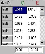
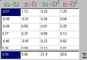 Just as we calculated the variance of a trait in the
first module, we can calculate the variance of these
two components in an identical manner. As shown in
the panel to the right, we simply take the deviations
from the mean (i.e. the first row, for G, is -0.514 - 0.061
= -0.57 after rounding), square them and then take the
average.
Just as we calculated the variance of a trait in the
first module, we can calculate the variance of these
two components in an identical manner. As shown in
the panel to the right, we simply take the deviations
from the mean (i.e. the first row, for G, is -0.514 - 0.061
= -0.57 after rounding), square them and then take the
average.