Help
LdOOKUP is designed to browse results from GWAS studies in a manner that is "LD (linkage disequilibrium) aware". The current instantiation hosts only GWAS data from the Psychiatric Genomics Consortium, alongside NHGRI GWAS catalogue summary results and brain eQTL data. (The underlying codebase is extensible however — feel free to contact us if you are interested in hosting your own LdOOKUP server.)
This page contains the following sections:
Underlying database
LD and variant information: Data from the 1000 Genomes project were used to calculate LD relations between all common autosomal, biallelic variants. Specifically, genotypes for founders (i.e. unrelated individuals) from the GBR, TSI and CEU subpopulations were extracted from the VCF files distributed by that project. For all variants with a combined minor allele frequency of 0.5% or greater, we calculated LD (using the --r2 function of PLINK. Considering pairs of variants within 1Mb, we recorded pairwise R-sq values of 0.3 or greater (thus for certain regions, e.g. MHC, long-range LD relations will not be captured). In total, from 11,573,447 biallelic variants (SNPs and indels) we recorded 655,695,743 pairs of variants in LD (R-sq > 0.3).
Variant identifiers: If a variant had an rsID, this was used as the primary identifier. Otherwise, we assigned a name in the form hg19:chr1:123456 and hg19:chr1:12345..12347 for indels where the reference allele is greater than one base. Queried variants must match the ID exactly. All matches are performed on the basis of the ID (i.e. not genomic position) All genomic coordinates are based on the hg19 reference sequence.
Genes: Gene definitions were based on UCSC canonical known gene track, downloaded from the UCSC Table Browser, and mapped to RefSeq transcript IDs and gene symbols.
GWAS results: Finally, GWAS summary statistics were obtained from the PGC and NHGRI websites and from Kim et al. (2014) and collated into the database.
Basic usage
The LdOOKUP database can be queried in one of three ways:
- Search on a gene symbol: this will list all variants within that gene and also all variants in LD with those genic variants
- Search on a variant: this will list information for this variant and all other variants in LD with this variant
- Collate a set of external results: this will take a list of results (e.g. from an independent GWAS), find all matching variants and variants in LD and collate and tabulate results across all GWAS
We will also add a search by region function in the near future.
GWAS datasets: Specific stored GWAS results can be included or excluded by checking each set (i.e. the list of stored GWAS in at the top-right corner of the page).
LD clumping: In each case, variants are first clumped to form groups of variants in high LD, using an on-the-fly algorithm. This algoirthm aims to group sets of SNPs that are in strong to moderate LD in order to provide a more interpretable description of associations across regions. Note that variants in different clumps are not necessarily statistically independent, however. That is, a single association signal may be represented as two or more clumps, but this does not necessarily mean that there are two independent association signals in that region. Specifically, LdOOKUP does the following:
- For a single variant (or for each variant in a gene/region), find all other variants in LD (R-sq>0.3), denoted here as LD friends.
- Group all LD pairs from (1) and consider each pair in order of decreasing R-sq.
- For each LD pair, considering variants denoted A and B
- if neither A nor B are already assigned to a clump, create a new clump containing A, B and all LD friends of A and all LD friends of B
- if A is already assigned to a clump but B is not, assign B and all LD friends of B to A's clump
- vice versa, if B is assigned but A is not
- if both A and B are already assigned to a clump, there is nothing further to do for that pair
- Finally, group any singletons (variants without any LD friends in the database) to a special singleton group (i.e that will contain variants not in LD with eachother unlike all other clumps).
Example: gene search
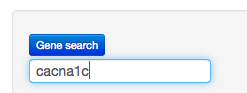
To search for results for the gene CACNA1C, enter the gene symbol in the gene search box:
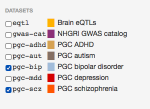
In these examples, we will just select results from the PGC schizophrenia and bipolar disorder studies: select these by checking the boxes in the right panel:
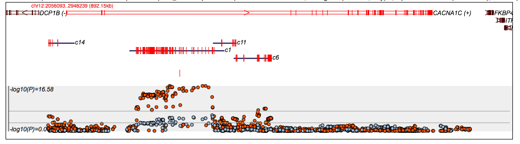
Then press the blue Gene Search button. You should then see a graphic depicting the gene(s) in the area including CACNA1C and information about association and LD:
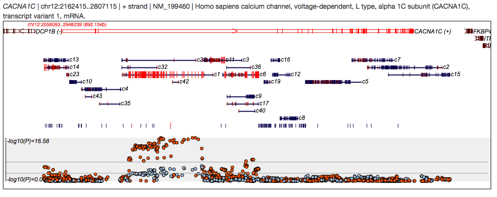
The gene figures show the exons (small vertical ticks) and strand orientation (arrow in middle and +/- labels). The query gene is shown in red. Below, the clumps of variants (those in strong LD) are depicted, and given arbitrary numbers (so they can be referenced in the table below). Red lines indicate significant associations (for at least one of the traits listed). Variants that are not assigned to a clump, or variants that belong to small clumps are shown separately in the row of ticks between the clumps and the association plot.
The bottom panel shows the association results (-log10(P)). Here the colours of the dots correspond to the legend in the top right (i.e. here, orange is PGC SCZ, blue is PGC BP).
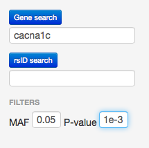
You can select to show only variants that are significant a certain threshold, e.g.:
which results in a more sparse plot:
Below the plot is a table of results. Each main row corresponds to a single clump; clumps can be expanded to show all SNPs by clicking on the Show/Hide labels. This clump therefore contains 87 SNPs that vary in frequency between 0.09 and 0.48. The index SNP is rs7980160. You can click on the blue links for variants and genes to search on those also.
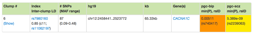
As mentioned, clumps are not defined to be statistically independent. The inter-clump LD information shows that this clump (labeled '6' is in LD with another SNP in a different clump ('11'). (In the future, we may add a more comprehensive clump-by-clump representation of LD, to make the interpretation of signals easier.)
The rightmost columns show the most significant P-values for the selected traits, from all variants in the clump.
Clicking on the Show link expands the table to the variant-level:
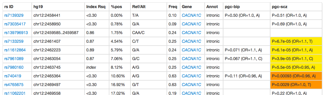
The Index Rsq field shows the LD between this SNP and the index SNP. This will typically be high, although a value of less than 0.3 (currently the minimum LD threshold) indicates that this variant was in strong LD with another variant that is in strong LD with the index. The %pos column indicates the physical location in the genomic interval spanned by the clump.
Variants that are nominally associated are coloured orange (P<0.05) or yellow (P<1e-4). If there was no result for that variant for a given GWAS, the cell will be blank.
Example: variant search
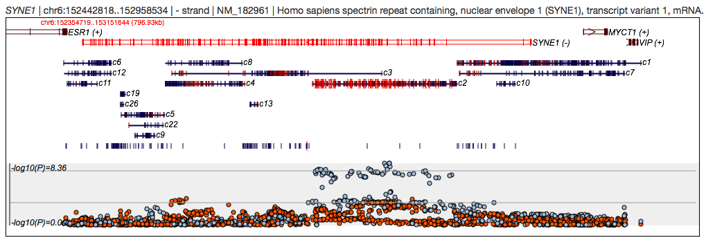
First, consider another gene search, on SYNE1, as shown here:
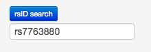
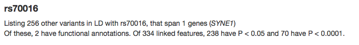
One of the associated variants is rs70016 - here we perform a variant search:
The results show that there are 256 other variants in the database that are in LD with this variant, along with the number of 'annotated' variants (i.e. nonsyn coding variants) and GWAS associations:
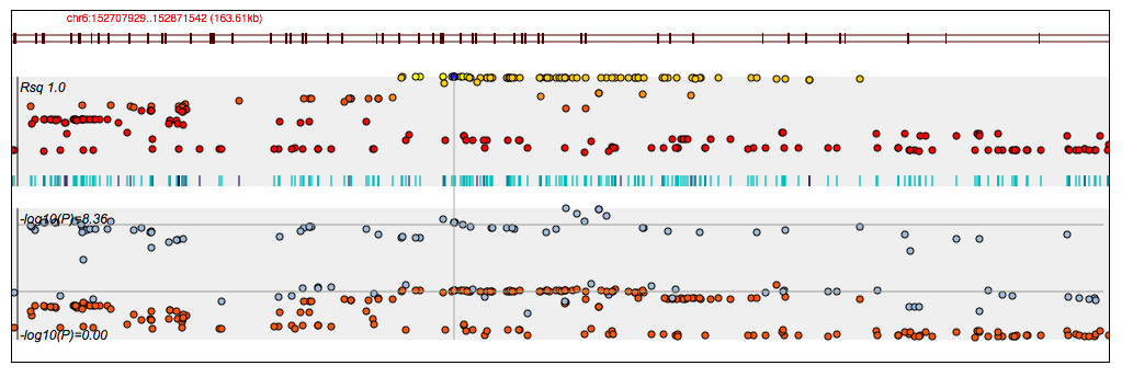
The plot below illustrates the LD centered around the key SNP (in blue); the bottom panel shows the Manhattan plot for the PGC SCZ and BP studies. (Note: the colours in the LD plot represent the strength of LD, rather than relating the to GWAS legend.)
Prioritized variants (those with a nominally significant result, or function coding SNPs) are shown below:
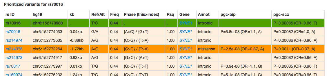
The variants here are ordered by decreasing LD with the index variant. Here we see, for example, that a missense SNP (rs214976) is in very strong LD with the query SNP.
(Note: LD was not calculated from the exact same sample as used in the different GWAS - that is, here we use the 1000 Genomes data as a common reference. Because of this, and also because of the application of imputation, you may see variants that have different P-values but Rsq values listed here as 1.00. Unless the difference in association results is very large, this should not be a cause for concern.
Example: collating results
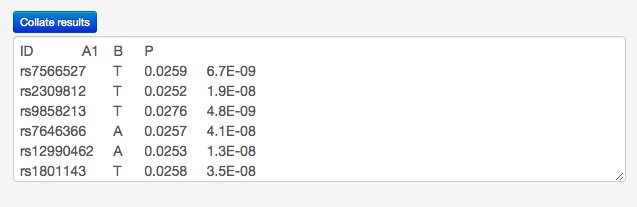
For this example, here we use publicly-available data from the Social Sciences Genetic Association Consortium (SSGAC); specifically, the first-stage meta-analysis for cognitive performance from Rietvald et al. (2014). Taking all variants with a P-value less than 5e-8, we obtain 92 variants, listed below along with the A1 allele and direction/size of effect given by the standardized beta (B):
ID	        A1	B	P
rs7566527	T	0.0259	6.7E-09
rs2309812	T	0.0252	1.9E-08
rs9858213	T	0.0276	4.8E-09
rs7646366	A	0.0257	4.1E-08
rs12990462	A	0.0253	1.3E-08
rs1801143	T	0.0258	3.5E-08
rs6750097	T	-0.0257	8.7E-09
rs11123817	T	0.0256	9.8E-09
rs11693324	T	-0.0254	1.3E-08
rs13013169	A	-0.0259	6.6E-09
rs11711485	T	0.0259	3.4E-08
rs4851264	T	-0.0260	5.6E-09
rs11689199	A	-0.0254	1.5E-08
rs2172252	A	-0.0269	1.4E-08
rs6446272	A	0.0260	2.6E-08
rs7608424	T	0.0240	4.1E-08
rs9837341	A	-0.0273	8.6E-09
rs9814873	A	-0.0261	2.7E-08
rs12994592	T	-0.0250	2.6E-08
rs6770670	T	-0.0263	2.9E-08
rs4851270	T	-0.0254	1.3E-08
rs6809216	A	0.0265	2.3E-08
rs1487441	A	0.0264	1.8E-09
rs1465800	T	-0.0256	9.7E-09
rs13026143	T	0.0253	1.8E-08
rs11685491	A	-0.0251	2.1E-08
rs11706370	A	0.0261	1.7E-08
rs13034176	A	0.0254	1.3E-08
rs3811697	T	0.0257	3.7E-08
rs2871344	A	-0.0260	5.8E-09
rs12615145	T	0.0256	1.4E-08
rs4583487	T	0.0255	1.0E-08
rs1160542	A	0.0256	4.3E-09
rs1122231	T	0.0254	1.3E-08
rs9841110	C	-0.0258	3.7E-08
rs1465801	T	0.0257	8.7E-09
rs9858542	A	0.0261	3.5E-08
rs11689201	A	-0.0260	4.9E-09
rs9858280	T	-0.0263	2.4E-08
rs12991254	T	-0.0259	6.6E-09
rs12614880	A	-0.0250	2.8E-08
rs13026283	T	0.0256	1.1E-08
rs9320913	A	0.0260	2.7E-09
rs4851266	T	0.0258	7.2E-09
rs6709656	A	-0.0259	6.6E-09
rs12202969	A	0.0258	3.4E-09
rs3811699	T	-0.0256	3.9E-08
rs10865035	A	-0.0256	4.9E-09
rs6766131	T	-0.0255	4.2E-08
rs13010010	T	0.0245	3.9E-08
rs4625	        A	-0.0255	4.2E-08
rs11718165	A	-0.0264	2.8E-08
rs6997	        T	0.0255	4.8E-08
rs11695383	T	0.0254	1.3E-08
rs4851267	A	0.0257	9.1E-09
rs12619178	T	0.0256	9.9E-09
rs11676922	A	0.0261	2.9E-09
rs11686372	A	0.0249	2.0E-08
rs999052	T	0.0257	8.6E-09
rs13401104	A	-0.0319	2.7E-08
rs6712515	T	-0.0262	2.2E-09
rs12053126	A	0.0255	1.3E-08
rs9653442	T	0.0256	4.7E-09
rs6803222	T	-0.0274	7.5E-09
rs9875617	A	0.0267	1.5E-08
rs1873625	A	0.0273	7.7E-09
rs9822268	A	0.0261	3.9E-08
rs11709525	T	0.0264	2.6E-08
rs9837027	T	0.0262	2.3E-08
rs9827708	C	-0.0269	1.2E-08
rs11922013	C	0.0257	4.6E-08
rs1987628	A	0.0260	2.6E-08
rs7633271	T	-0.0258	3.3E-08
rs2309838	T	-0.0255	1.1E-08
rs13017207	A	0.0252	2.2E-08
rs11123818	A	0.0253	1.7E-08
rs11687241	A	-0.0256	1.0E-08
rs12206087	A	0.0259	3.0E-09
rs9823546	A	0.0260	5.0E-08
rs1800668	A	0.0261	2.9E-08
rs1906252	A	0.0255	4.9E-09
rs1160543	T	0.0252	1.7E-08
rs10865037	T	-0.0245	4.4E-08
rs11695996	T	0.0251	2.1E-08
rs11684761	A	0.0254	1.3E-08
rs10496345	T	-0.0260	5.5E-09
rs4851271	T	-0.0254	1.2E-08
rs9827021	A	0.0258	3.6E-08
rs11130213	T	0.0264	2.3E-08
rs7622302	T	-0.0258	4.0E-08
rs10496346	A	0.0252	2.0E-08
rs893246	T	-0.0260	5.7E-09
Copy the above lines (including the header row), paste them into the Collate results textbox of LdOOKUP and press the Collate results button. An ID (or RSID) field is required; all other fields are optional (and fields other than P, A1 and B can be included). Fields should be white-space delimited; there should be the same number of fields on each row.
Press the Collate results button, and you should see the following table:
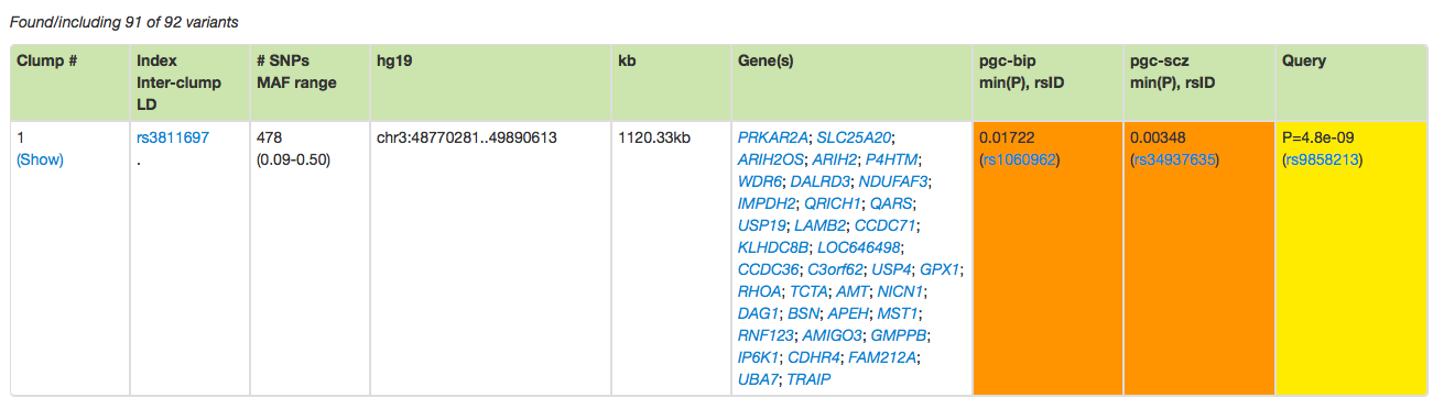
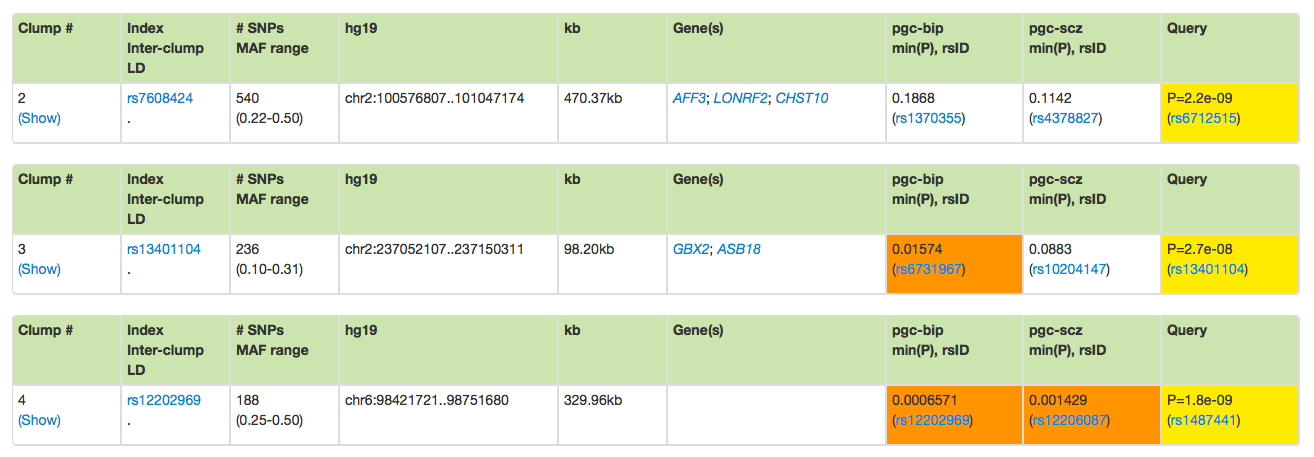
This is the first of four rows, indicating that these 92 variants (91 of which were found in the database) can be grouped as four clumps.
As with the genic search, you can click on Show to see variant-level results, which shows the query SNPs, but also all variants in the database that are in LD with the query SNPs:
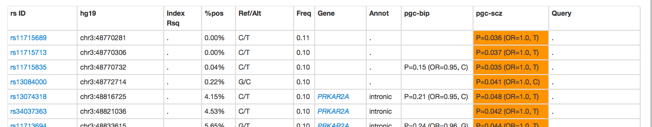
Any rows that are shaded gray were in the original query - these SNPs will have the data from the original query (i.e. the P, B and A1 fields) listed in the rightmost Query column:
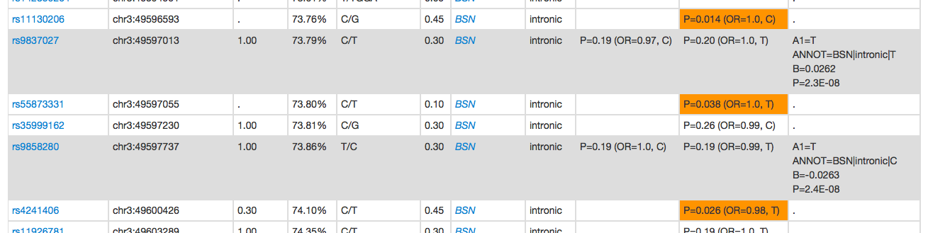
Care is still needed in interpreting whether different association results are concordant across studies. In this example, although this first clump has nominally significant variants for all three traits, when looking at the specific variants driving the signals, those associated in SCZ and BP are typically different from those associaited with cognition, despite the low/moderate level of LD between all SNPs (i.e. why they were clumped in the first place).
Finally, the three other clumps are shown below. In this example, the 92 variants have been
grouped into four clumps. The absence of Inter-clump LD informtion (.) indicates that these clumps
are relatively independent.
Known issues
- X/Y chromosome variants currently not included
- The release of 1000 Genomes data used to calculate LD is missing some genomic regions -- this will be corrected in the near future, when new 1000 Genomes releases are available
- When using the input form, pressing return (rather than clicking a submit button) will always perform a gene-search. Thus, one should always click on the specific blue button rather than press return to submit the form.
- The included studies are only updated after clicking one of the three submit buttons -- i.e. not after clicking on a variant or gene link in the report tables. Thus, if one changes the included studies (by changing the checkboxes in the top right of the screen), this change will not be taken into effect unless followed by a search initiated by pressing one of the three blue submit buttons.
- A feature to query a region rather than a gene/variant will be added in the near future
- Note that when collating results across GWAS, LdOOKUP implicitly assumes that all alleles are encoded with respect to the positive strand.
Creating a databse
Currently, these notes are primarily for our own refernce -- at this moment we are not distributing the codebase for LdOOKUP. If you are simply querying an existing website, you can ignore all the information below.
Creating a new database
All data are hosted in a single file/database and should be imported in the following steps. Except where noted, all imported files are expected to be tab-delimited rectangular files.
If the primary database is to be called main.db, first ensure we are starting from a blank database:
rm -rf main.db
Primary variant table
Import the full set of known variants. All variants are identified based on the ID or RSID field in this file. Any variants subsequently found in GWAS summary files, or in user queries, or ignored if they are not present in this file.
./ldookup variant-table main.db < dbsnp.txt
The file dbsnp.txt should have the following type of format:
RSID            CHR     BP      REF     ALT     ANNOT                 FRQ      NSF     NSM     NSN     SYN     U3      U5      ASS     DSS     INT     R3      R5
rs145072688     1       10352   T       TA      .                     0.4375   .       .       .       .       .       .       .       .       .       .       +
rs200579949     1       13118   A       G       DDX11L1|intronic|G    0.097    .       .       .       .       .       .       .       .       +       .       .
rs75454623      1       14930   A       G       WASH7P|intronic|G     0.4822   .       .       .       .       .       .       .       .       +       .       .
rs199856693     1       14933   G       A       WASH7P|intronic|A     0.0284   .       .       .       .       .       .       .       .       +       .       .
Required fields: The only required fields are RSID (or equivalently ID), CHR and BP (or BP1 and BP2), REF and ALT. The ALT field should be a comma-delimited list of non-reference alleles. If present, the field FRQ is treated in a special manner, taken to be the combined frequency of all non-reference alleles (i.e. as tabulated in the query output).
Special annotation codes: Some fields are interpreted as special annotation features. As well as FRQ and the other fields described above, ANNOT fields specify variant annotations in the following "|"-delimited manner: gene|annotation|alt-allele.
Tags: Features with values of . or + are interpreted as tags rather than key/value pairs -- only values with + will be stored and displayed.
LD information
./ldookup ld-table main.db < ld.txt
The file ld.txt should have the format: 4 tab-delimited columns, no header, that list the two variant IDs, the allele coupling (i.e. which haplotypes are over-represented) and the R-sq.
rs116400033      rs141149254       A|A/T|G  0.76757
rs116400033      rs138808727       A|T/T|A  0.717088
rs116400033      rs147061536       A|T/T|G  0.728617
hg19:chr1:51762  hg19:chr1:51765   G|G/A|C  1
rs150021059      hg19:chr1:52253   T|G/G|C  0.49481
...
That is, the first line implies that rs116400033 is an A/T SNP, rs141149254 is a A/G SNP, and the haplotypes AA and TG are more common (i.e. A is associated with A and T is associated with G).
Genes
Gene information is stored in following tab-delimited format:
genes   UCSC canonical transcripts (hg19)
CHR     BP1     BP2     ID      REFSEQ          DESC                                                                                 STRAND  EX1                                                                                                  EX2
chr1    69090   70008   OR4F5   NM_001005484    Homo sapiens olfactory receptor, family 4, subfamily F, member 5 (OR4F5), mRNA.      +       69090,                                                                                               70008,
chr1    367658  368597  OR4F29  NM_001005277    Homo sapiens olfactory receptor, family 4, subfamily F, member 29 (OR4F29), mRNA.    +       367658,                                                                                              368597,
chr1    621095  622034  OR4F29  NM_001005277    Homo sapiens olfactory receptor, family 4, subfamily F, member 29 (OR4F29), mRNA.    -       621095,                                                                                              622034,
chr1    861120  879961  SAMD11  NM_152486       Homo sapiens sterile alpha motif domain containing 11 (SAMD11), mRNA.                +       861120,861301,865534,866418,871151,874419,874654,876523,877515,877789,877938,878632,879077,879287,   861180,861393,865716,866469,871276,874509,874840,876686,877631,877868,878438,878757,879188,879961,
All fields are special, required fields. The EX1 and EX2 fields contain the exon start/stop positions (comma-delimited list). Note that the first line must contain two tab-delimited fields and the first word must be the term genes in order for this file to be specially interpreted as the gene track (i.e. as opposed to another generic "feature").
The following command will then import the gene track:
./ldookup gfeature-table main.db < glist-hg19.txt
Features
Each GWAS summary dataset should be a standard tab-delimited file; the only required field is ID (or RSID). Any positional (CHR, BP, etc) information is not treated specially -- i.e. the positional information is taken from the the initial variant file. Special fields are A1 (the non-reference allele, i.e. such that is the odds ratio is greater than 1.0, then A1 is the risk-increasing allele). The A1 allele need not be the minor or reference allele; by convention however, all alleles should be reported on the positive strand.
As with the gene file, the first row should contain exactly two tab-delimited fields: a short name and a full name. The second row should be the header row; all subsequent rows should have the same number of fields.
gwas1   Disease X
ID      A1      OR      P
rs4951859       C       0.97853 0.2083
rs142557973     T       1.01949 0.3298
rs141242758     T       1.02071 0.3055
rs79010578      A       0.98748 0.5132
To import the above information:
./ldookup feature-table main.db < gwas1.txt
Other fields can be present -- these will be stored (and reported) as additional pieces of information in subsequent reports.
Setting up the webserver
LdOOKUP expects two valid links/files in the directory in which is it hosted/executed:
- lookup.cgi : the primary C/C++ code
- lddb.db : the database
For example, if hosting LdOOKUP from http://my.server.org/ldookup/ and ~/www/ is the HTML root, and the ldookup.cgi binary is in ~src/ldookup/, and the database is called main.db and located in ~/working/ldookup/data/ then:
mkdir -p ~/www/ldookup
cd ~/www/ldookup
ln -s ~/working/ldookup/data/main.db lddb.db
ln -s ~/src/ldookup/ldookup ldookup.cgi
You may also want to add a page to redirect from the primary index.html, e.g.:
<html>
<head>
<meta HTTP-EQUIV="REFRESH" content="0; url=http://my.server.org/ldookup/ldookup.cgi">
</head>
<body></body>
</html>