
Univariate Twin AnalysisS.Purcell, 2000.
IntroductionIn this tutorial we shall take a look at a dataset containing scores for 500 MZ twins and 500 DZ twins on a single measure. The aim of these particular analyses is to determine whether or not there is any evidence for a genetic effect on the trait. The dataset can be downloaded here. Depending on your browser, you might have to right-click and choose 'Save As...' or 'Save Target As...'. Alternatively, you might be able to left-click on the link to view the raw data in your browser window and then copy-and-paste the dataset into WordPad or some other text-editor and save it from there onto your computer. The dataset is in comma-separated value format so it can be read by almost any program, including Excel. Each row of the dataset represents information on one twin pair. It contains four variables:
 If you have access to Stata, open it up, after you have transfered
the datafile to your computer. If you do not have access to
Stata, open up whichever statistics package you are most
familiar with. A spreadsheet such as Excel could even be used
for most of these analyses.
In the Stata command line, type the following to load the
raw data into memory, replacing the u:\ path with
the appropriate path for your computer. The comma
option after the filename tells Stata to expect a
comma-separated value file.

 Assuming it loads correctly, you should see the following
text in the output window. This simply confirms the fact
that our data file contains 4 columns (i.e. the variables
as listed above) and 1000 observations (i.e. 500 MZ twin pairs
and 500 DZ twin pairs).
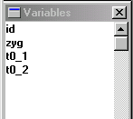 The Variables window in Stata should display the
names of the four variables. These were the top row of the
raw datafile (often called the header row). Unlike SPSS,
Stata does not provide a spreadsheet-style view of the data
by default. Although it can sometimes be useful to literally
see all your data on the screen, when working with large
datasets, as is typical in quantitative genetic research,
the spreadsheet-style view becomes less useful.
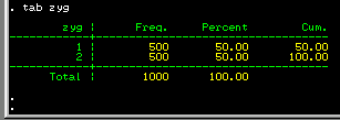 The tab command in Stata is used to tabulate
values of a variable to produce a frequency table. Type in
tab zyg to get a breakdown of the zygosity status
of the sample. If all is well, this should confirm that you
have successfully loaded 500 pairs of each twin zygosity
into Stata.
The trait scores for each twin (t0_1 and t0_2)
are continuously-distributed variables, so it is not informative
to tabulate each the values in the same manner as above.
Rather, we have to rely on summary descriptive statistics
such as the mean and variance to tell us about the distribution.
The command su (summarise) can be used to give these
statistics. If you type su t0_1 t0_2 Stata will
print the mean for all twin 1s and all twin 2s separately,
as well as several other useful statistics such as the
standard deviation.
 We can see that there is no real
difference between the mean scores for all twin 1s and all
twin 2s. Also, there is no real difference in the variability
of these variables: the standard deviations are very similar.
Another useful way to look at data is to plot it. To
generate a histogram for all twin 1 scores, type the
following:
 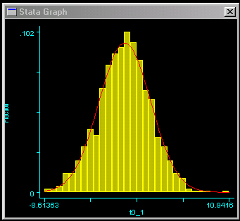 This should result in the graph as shown to the right. We can
see that the trait is approximately normally distributed, which
is good news for these analyses.
In genetic analyses, we are often more concerned with the relationships in scores between related individuals. An ideal way to get a sense of the relationship between two continuously-distributed measures is to draw a scatter-plot of the two variables. We can use the following command to plot the scores of one twin against the scores of the other twin.  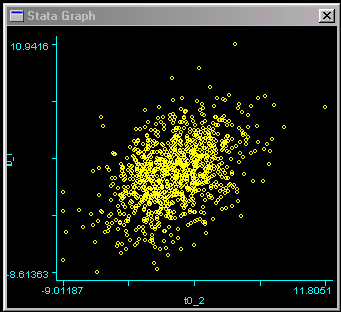 Each dot represents a twin pair: the position on the vertical,
or y, axis represents the score for the first twin,
the position on the horizontal, or x, axis represents
the score for the other twin. We can see evidence of an
association between twins here: the distribution is slightly
more drawn-out going from bottom-left to top-right. That is,
individuals who score low are more likely to have co-twin
who also scores below average, and vice-versa. The association
is by no means strong, however.
 We can quantify this association between scores with a
correlation coefficient. Type the command as shown
to the right for Stata to calculate the correlation between
twins for this trait.
 Stata displays the following correlation matrix: the
correlation is 0.4241. This will undoubtably be significantly
greater than zero (the command pwcorr t0_1 t0_2, o sig
can be used to also give p-values for the correlations).
So far, all the graphs and statistics have not differentiated
between MZ and DZ twins. The aim of this analysis is to
compare twin similarity between MZ and DZ twins, so we
need to analyse twins separately by their zygosity.
Type the command sort zyg to sort the dataset by
this variable. It is now possible to stratify
analysis by twin zygosity. That is, rather than giving
the twin correlation for all twins, Stata will output
the twin correlation for MZ twins and DZ twins separately.
 Looking first at whether there are any differences in means
or standard deviations between MZ and DZ twins, use the
command as shown to the right.
 The output of this command, shown left, is now broken down for MZ
and DZ twins: we can see that there is no big difference
between MZ and DZ twins in terms of their trait means or
standard deviations. (Formally, we would test these
statistically, but an 'eye-ball test' will suffice for
present purposes.)
 Now enter the following command, shown to the right, in
order to obtain the twin correlations for MZ and DZ
twins separately: these quantities are fundamental to
the twin analysis we are about to perform.
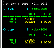 We see that the MZ correlation (0.5231) is larger than the
DZ correlation (0.3204). So the correlation we obtained
earlier for the whole sample, ignoring twin zygosity,
effectively represented an average between these two
figures.
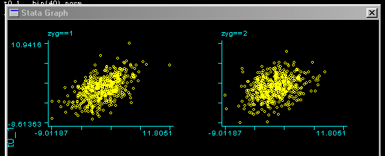
Looking at the scatter-plots by zygosity we can see this
difference in correlations: the left scatter-plot is
for MZ twins, the right one for DZ twins. We can see a
slightly stronger relationship for MZ twins.
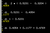 We can use the di (for display) command in Stata
to act as a pocket calculator: the estimate for heritability
is therefore approximately 40% (i.e. twice the difference
between MZ and DZ correlations is 0.4054). The shared
environment accounts for 12% of variation, whilst nonshared
environmental effects account for just under half of the
variance in this population. The last line merely confirms
that these proportions of variance do in fact add up to 1,
as they should
Covariances and Model-fitting These estimates of heritability are based on the comparison
between correlations. As mentioned in the Appendix, it is
often preferable to analyse variances and covariances instead,
for a number of reasons. We can obtain the variance-covariance
matrices for MZ and DZ twins from Stata by adding the cov
option to the correlation command as shown to the right.
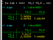 As we saw earlier, there are no major differences between four
estimates of variance. We can apply model-fitting methods to these
variance-covariance matrices and compare the results to the simple
analysis with correlations.
We can use the Model-fitting 2 module from the main BGIM site. Clicking on the WWW symbol shown below enters the module designed to perform model-fitting analysis on univariate twin data. 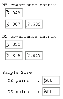 We can simply enter the MZ and DZ variances and covariances estimated
by Stata into this module: the picture to the right shows these.
Also, we must specify how many MZ and DZ twins these variances
and covariances were based on - 500 each in this case. Not
shown here, the module also asks for a Type I error rate :
just enter 0.05 for this. This represents the
chance of falsely rejecting a model, as described in the Appendix
and other modules.
The results of this analysis are shown below:  The figures represent components of variance. From the full
ACE model we obtain a similar estimate of heritability as from
the correlational analysis. The total variance is 2.7124 + 1.122 +
3.6693 = 7.4937. Therefore the proportion of variance due to
additive genetic effects, or heritability, is 2.7124/7.4937 = 0.36.
In other words, the model-fitting analysis estimates that 36% of the
variation in the population is due to genetic effects. This can be
regarded as a more accurate estimate than the 40% obtained from
analysing correlations. The reason for the difference is that the
model-fitting analysis is taking into account the small differences amongst
the four variances.
We also see that the best-fitting model is in fact the AE model: that
is, the effect of shared environment is not significant. A model with
only additive genetic and nonshared environmental effects is shown on
the second line (again, go to the module tutorial for a full explanation
of all the figures in this table). The standard estimates from the AE
model are given below: the impact of genes is estimated much higher
now:

Further exploration: SimulationThe datafile we used in the analysis above was not collected from real individuals measuring any particular trait: it was simulated, using the SIMULATOR module at this website.

 By selecting the Calculate option, the module gives the
corresponding proportions of variance attributable to A, C and E.
In this case the total variance is there therefore 9 (2*2 + 1*1 + 2*2).
The proportion of variance due to additive effects of genes is
(2*2) / 9 = 44.4%. In a similar manner, we calculate that the shared
environment accounts for 11.1% of variance, the nonshared environment
for 44.4%.
In infinitely large samples, the methods of
analysis used here would have yielded these exact figures. Instead, because
of sampling error, the estimates were slightly off, even though
the sample sizes seemed reasonably large.
Try using the simulation module to create another dataset
according to the same properties, analyse it, and you will
notice that the estimates will be slightly different again.
But if you repeated this a large number of times, you should
also notice that the estimates may be a little out each time,
but there should be no consistent bias in them (i.e. such as
the heritability being consistently over-estimated).
Bear in mind, however, the simulation module simulates data
according to very simplistic assumptions that might not
hold in real life, which potentially could lead
to systematic bias. An example of this would be the equal
environment assumption, as mentioned in the Appendix.
Try simulating a univariate dataset with different
values, and then use Stata to calculate the correlations
and covariances. Try experimenting with the approximate
size of samples you need before the estimate become stable.
Further exploration: Using Mx to perform the analysisTry installing Mx on your computer and run the basic ACE script to perform the same analyses. The basic ACE script can be found here. You will need to edit the script just to enter the covariance matrices, as follows:
Group2: MZ twin pairs
Data NInput_vars=2 NObservations=500
     CMatrix
	7.949
	4.088 7.682
and for DZ twins
Group3: DZ twin pairs
Data NInput_vars=2 NObservations=500
     CMatrix
	 7.012
	 2.315 7.447
Looking at the output, you will see the relevant parameters A, C and
E representing the components of variance. These will correspond very
closely to the values obtained from the model-fitting module above.
In this case,
  MATRIX A
 This is a computed FULL matrix of order    1 by    1
  [=X*X']
             1
 1      2.7139

  MATRIX C
 This is a computed FULL matrix of order    1 by    1
  [=Y*Y']
             1
 1      1.1213

  MATRIX E
 This is a computed FULL matrix of order    1 by    1
  [=Z*Z']
             1
 1      3.6684
The script also contains a standardisation group, so the proportions
of variance are also given (T, U and V correspond to A, C and E
respectively).
  MATRIX T
 This is a computed FULL matrix of order    1 by    1
  [=D~*A*D~]
          1
 1   0.3617

  MATRIX U
 This is a computed FULL matrix of order    1 by    1
  [=D~*C*D~]
          1
 1   0.1494

  MATRIX V
 This is a computed FULL matrix of order    1 by    1
  [=D~*E*D~]
          1
 1   0.4889
This gives the same heritability estimate, 36%. The fit statistics
are also important:
 Your model has    3 estimated parameters and      6 Observed statistics

 Chi-squared fit of model >>>>>>>     1.984
 Degrees of freedom >>>>>>>>>>>>>         3
 Probability >>>>>>>>>>>>>>>>>>>>     0.576
The non-significant fit (p=0.576) represents that the model accounts for the observed data well. The script can be modified to test an AE model- remove the free keyword after the Y matrix from the first group: Begin Matrices; X Lower nvar nvar free ! genetic structure Y Lower nvar nvar ! shared environment Z Lower nvar nvar free ! non-shared path co-efficients H Full 1 1 End Matrices;As can be seen this gives similar results to the model-fitting module above:
  MATRIX T
 This is a computed FULL matrix of order    1 by    1
  [=D~*A*D~]
          1
 1   0.5252

  MATRIX U
 This is a computed FULL matrix of order    1 by    1
  [=D~*C*D~]
          1
 1   0.0000

  MATRIX V
 This is a computed FULL matrix of order    1 by    1
  [=D~*E*D~]
          1
 1   0.4748
Try using Mx to test the CE model; try analysing other univariate
twin covariance matrices.
The next tutorial will consider the multivariate extension
to these analyses.

Site created by S.Purcell, last updated 30.11.2000 |
||||


