Behavioural Genetic Interactive Modules

Families
Overview
This module is designed to illustrate the
ways in which the different sources of variation in a trait (genetic
and environmental) result in particular patterns of expected
correlations between related individuals.
Tutorial
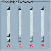 Upon loading the module you will see three main panels.
The top two panels are both labelled Population Parameters.
The left panel contains three sliders labelled A, D,
C and E which correspond to additive genetic,
dominance genetic, shared (common) environment
and nonshared environment components of variance respectively.
These four components of variance represent the relative balance
of nature and nurture for a particular trait. This trait could
be any continuous measure such as height, IQ or severity of anxiety
symptoms. These sliders are used to control the relative balance
of influences on the trait.
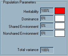 The panel to the right represents the percentage of total variance
that each of these four components accounts for. We assume that
the variation in the trait (including measurement error) is completely
accounted for by these four latent variables and so these four
percentages will always sum to 100%. Moving the sliders results
in a corresponding change in these figures.
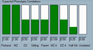 The panel
at the bottom of the window contains a graphical and numerical
display of the correlations that we would expect to observe for
the trait, if the trait had the relative balance of genetic and
environmental effects specified in the top panel (i.e. 100% heritable).
The leftmost column is labelled Proband, the "correlation"
between individuals and themselves. Of course, this correlation
will always be a complete positive correlation of 1.0 (the maximum
possible correlation). In the second column, the height of the
green bar and the number below represents the correlation we
would expect to observe between MZ twins. Likewise, the next
three columns represent the correlations we would expect to see
between DZ twins, full siblings and parent-offspring. The next
two columns represent the expected correlations for MZ and DZ
twins reared apart (i.e. no shared environment, but still shared
genes). The correlation for half-siblings (half siblings raised in
the same family) is next; finally, the
expected correlation between the proband and any unrelated individual
chosen at random is shown. The panel
at the bottom of the window contains a graphical and numerical
display of the correlations that we would expect to observe for
the trait, if the trait had the relative balance of genetic and
environmental effects specified in the top panel (i.e. 100% heritable).
The leftmost column is labelled Proband, the "correlation"
between individuals and themselves. Of course, this correlation
will always be a complete positive correlation of 1.0 (the maximum
possible correlation). In the second column, the height of the
green bar and the number below represents the correlation we
would expect to observe between MZ twins. Likewise, the next
three columns represent the correlations we would expect to see
between DZ twins, full siblings and parent-offspring. The next
two columns represent the expected correlations for MZ and DZ
twins reared apart (i.e. no shared environment, but still shared
genes). The correlation for half-siblings (half siblings raised in
the same family) is next; finally, the
expected correlation between the proband and any unrelated individual
chosen at random is shown.
The only controls in this module are the
four sliders in the top left panel. Moving the A slider
up increases the relative proportion of trait variance attributable
to additive genetic variation. Because all the other parameters
are set to zero, this will suddenly jump to 100%. That is, the
value for Heritability given in the top right panel will
read 100%, indicating that the trait is completely determined
by the additive effects of genes.
Looking at the expected correlations under
this somewhat unrealistic scenario, we see that they represent
the expected proportion of allele sharing for the different types
of relatives. Because MZ twins share all their genes, then if
the trait is completely determined by additive genetic effects,
MZ twins will correlate completely for the trait. DZ twins, full
siblings and parent-offspring pairs, all of whom share only half
their alleles, are only expected to show a correlation of 0.50.
Because this simple model states no environmental effects, twins
reared apart are expected to be just as similar to each other
as those reared together.
We would be very unlikely to ever see this
pattern of correlations in families for any complex behavioral
trait. For certain Mendelian traits with complete penetrance,
we might observe a pattern of familial correlations close to
this. Given that measurement error is incorporated into the nonshared
environmental component of variance, it is extremely unlikely
that this will ever be zero.
So try sliding the nonshared environment
E control upwards. Note what happens: in the top right
window we can see that the magnitude of the nonshared environmental
component increases and all of the expected correlations
between family members drop.
Note that the familial correlations remain
in proportion with each other, however, when varying the E
component. That is, the DZ twin correlation always remains half
the expected MZ correlation, for example. Although the nonshared
environmental is now contributing to the variance of the trait,
it does not (by definition) contribute to the similarity between
family members. Under this scenario, what makes related individuals
similar is still completely the additive effect of genes, so
we would still expect similarity to reflect exactly the expected
proportion of allele sharing between relative pairs.
Now try increasing the C slider.
Note how some correlations rise and some fall, all at different
rates. It is the nature of this relationship, between the aetiological
components of variance and the expected familial correlations
that is the key to many quantitative genetic methods. Incorporating
dominance (the D slider) further influences the pattern
of expected correlations.
The expected correlations for each type
of relative pair are entirely determined by the four population
parameters. The Behavioral Genetics Appendix gives an account
of how familial correlations can be expressed in terms of the
sharing we would expect for variance components, which can be
derived from basic biology (for the genetic components) or by
definition (for the environmental components).
Questions
- The correlation bars only range between
0 and 1 but correlations can be negative. Why would we never
expect to observe a negative correlation between family members
if we assume this simple model is an accurate reflection of the
trait aetiology? (Note: In certain special circumstances we
might actually expect to observe negative correlations between
relatives (e.g. sibling interaction))
- The correlation between unrelated individuals
is always fixed at 0. Why is this?
- Is there any configuration of variance
components that makes every different type of relative pair have
a unique expected correlation? If not, why not?
- The expected correlation for full siblings
is calculated as half the additive genetic variance (heritability)
plus a quarter of the dominance genetic variance plus shared
environmental variance.
Set the population parameters to 20%, 12%,
20% and 48% for the heritability, dominance, shared environmental
and nonshared environmental variance respectively (note: this
can be a bit tricky, as moving one slider may cause one component
to increase but all the others also fall! This is because they
represent proportions and so must always sum to 1, i.e. 100%).
See that the expected correlation between
siblings is now 0.33. Check that this corresponds to the value
we would calculate using the information given above. At these
population parameter values, the expected correlation between
parent and offspring is 0.30. By moving the sliders and observing
the changes in these values, try to determine the rule that gives
the expected correlation between parent and offspring. Also,
what is it for half siblings?
- This module makes several assumptions that
we would not necessarily want to make in a proper analysis. One,
for example, involves the equal environment assumption.
Typically we assume that MZ and DZ twins share equally similar
environments; this modules extends this assumption to parents
and half-siblings however. That is, there is only one shared
environmental parameter for all the different types of relatives
in this module. Can you give an example of when this assumption
might not be valid?
Answers
- Under our model, the trait is composed
of four independent components: additive and dominance genetic
effects, shared and nonshared environmental effects. None of
these could, theoretically, induce a negative correlation between
family members (remember that nonshared effects do not tend
to make pairs of individuals dissimilar, rather they are
effects which make tend to make pairs of individuals neither
similar nor dissimilar). If a trait were entirely due to
nonshared environmental effects, then we would expect family
members to be just as similar (and alternatively, just as dissimilar)
as pairs of unrelated individuals.
Note that it might be possible to observe
a negative familial correlation in a sample if the nonshared
environmental variance is very high and the sample size is low.
In this case, the expected correlation would be positive
but near zero, but the small sample size would imply a large
degree of sampling error in the estimation of the correlation.
-
This correlation is by definition 0, which
means that, on average, we would expect to see no relationship
between unrelated individuals. Imagine that we chose 1000 pairs
of unrelated individuals at random and measured them for a particular
trait. If we found a negative correlation this would imply
that we had somehow managed to pair low scoring individuals with
high scoring individuals. If we found a positive correlation
this would imply that we had tended to pair high-scoring individuals
with high-scoring individuals, low-scoring with low-scoring.
If we do not expect either of these processes to occur (there
is no reason they should do if the sampling is random) then we
must expect a zero correlation. Note that this says nothing about
the level of variation in the population of unrelated individuals
for the trait. That is, whether or not the trait had a very large
or a very small variance, we would still expected unrelated individuals
picked at random from any population to display a zero correlation.
-
DZ twins and full siblings will always
have the same expected correlation under this model. In the eyes
of this model, DZ twins are just like normal full siblings. Genetically
speaking there is also no difference between DZ twins and full
siblings: DZ twins are siblings that just happen to have been
conceived at the same time. As question 5 indicates however,
there may be other reasons which suggest that equating DZ twins
and full siblings might not be sensible.
-
Parents and offspring also share half their
additive genetic variance but they do not share dominance genetic
variance. Half siblings share a quarter of the additive genetic
variance. Both types of relative pair share all shared environmental
variance (by definition) (although, typically, we would not expect
the magnitude of this to be the same for all different types
of relative pair - see question and answer 5).
-
One example would be if we were to study
young MZ and DZ twins and their parents for a trait such as bladder
control. The types of environment that tend to induce a correlation
between young twins for this trait would probably be quite different
from any environment that induced a correlation between parent
and offspring for this trait. Imagine that exposure to potty
training influences bladder control (and acts as a shared environmental
source of trait variance), for example.
Return
to Modules Menu
Site created by S.Purcell, last updated 6.11.2000
|

 Upon loading the module you will see three main panels.
The top two panels are both labelled Population Parameters.
The left panel contains three sliders labelled A, D,
C and E which correspond to additive genetic,
dominance genetic, shared (common) environment
and nonshared environment components of variance respectively.
These four components of variance represent the relative balance
of nature and nurture for a particular trait. This trait could
be any continuous measure such as height, IQ or severity of anxiety
symptoms. These sliders are used to control the relative balance
of influences on the trait.
 The panel to the right represents the percentage of total variance
that each of these four components accounts for. We assume that
the variation in the trait (including measurement error) is completely
accounted for by these four latent variables and so these four
percentages will always sum to 100%. Moving the sliders results
in a corresponding change in these figures.
 The panel
at the bottom of the window contains a graphical and numerical
display of the correlations that we would expect to observe for
the trait, if the trait had the relative balance of genetic and
environmental effects specified in the top panel (i.e. 100% heritable).
The leftmost column is labelled Proband, the "correlation"
between individuals and themselves. Of course, this correlation
will always be a complete positive correlation of 1.0 (the maximum
possible correlation). In the second column, the height of the
green bar and the number below represents the correlation we
would expect to observe between MZ twins. Likewise, the next
three columns represent the correlations we would expect to see
between DZ twins, full siblings and parent-offspring. The next
two columns represent the expected correlations for MZ and DZ
twins reared apart (i.e. no shared environment, but still shared
genes). The correlation for half-siblings (half siblings raised in
the same family) is next; finally, the
expected correlation between the proband and any unrelated individual
chosen at random is shown.