Video tutorial available here or on YouTube
How to run XHMM
After installation, run xhmm (with appropriate options):
./xhmm -p params.txt
where an example of params.txt is given below.
Download "toy" data set based on 1000 Genomes Project data
- Note that the following data can be used to run the workflow commands below, once you've installed the following:
-
The following external files also need to be downloaded:
Human reference genome files:
human_g1k_v37.fasta.gz, human_g1k_v37.fasta.fai from here -
Data files:
(163 MB zip file) 1000 Genomes BAM files for 30 sample across first 300 exome targets.- Note that full exome BAM files from the 1000 Genomes Project can be downloaded, for example, from http://ftp.1000genomes.ebi.ac.uk/vol1/ftp/data/HG00096/exome_alignment/HG00096.mapped.ILLUMINA.bwa.GBR.exome.20120522.bam
- OR, you can skip the GATK step for this example and use the GATK's DepthOfCoverage output for the above 30 samples
- Note: the standard params.txt file comes as part of the XHMM installation (in the highest-level directory).
- And, a barebones version of the R plotting script for this data set can be found here.
- And, for comparison, all files output by running the pipeline below (including the R plotting script) on this data are given here.
What does a "typical" XHMM workflow look like?
NOTE: It is assumed that the BAM files of "analysis-ready reads" being used have been generated using the "best practice" bwa + Picard + GATK pipeline, though variations on this pipeline, and even other pipelines to produce the BAM files for XHMM input, have been successfully employed by various users. For running GATK's DepthOfCoverage in parallel, first split up your samples' list of BAMs into the desired degree of parallelism (in the example here, three files): group1.READS.bam.list group2.READS.bam.list group3.READS.bam.list Run GATK for depth of coverage (three times: once for samples in group1, once for group2, and once for group3): java -Xmx3072m -jar ./Sting/dist/GenomeAnalysisTK.jar \ -T DepthOfCoverage -I group1.READS.bam.list -L EXOME.interval_list \ -R ./human_g1k_v37.fasta \ -dt BY_SAMPLE -dcov 5000 -l INFO --omitDepthOutputAtEachBase --omitLocusTable \ --minBaseQuality 0 --minMappingQuality 20 --start 1 --stop 5000 --nBins 200 \ --includeRefNSites \ --countType COUNT_FRAGMENTS \ -o group1.DATA java -Xmx3072m -jar ./Sting/dist/GenomeAnalysisTK.jar \ -T DepthOfCoverage -I group2.READS.bam.list -L EXOME.interval_list \ -R ./human_g1k_v37.fasta \ -dt BY_SAMPLE -dcov 5000 -l INFO --omitDepthOutputAtEachBase --omitLocusTable \ --minBaseQuality 0 --minMappingQuality 20 --start 1 --stop 5000 --nBins 200 \ --includeRefNSites \ --countType COUNT_FRAGMENTS \ -o group2.DATA java -Xmx3072m -jar ./Sting/dist/GenomeAnalysisTK.jar \ -T DepthOfCoverage -I group3.READS.bam.list -L EXOME.interval_list \ -R ./human_g1k_v37.fasta \ -dt BY_SAMPLE -dcov 5000 -l INFO --omitDepthOutputAtEachBase --omitLocusTable \ --minBaseQuality 0 --minMappingQuality 20 --start 1 --stop 5000 --nBins 200 \ --includeRefNSites \ --countType COUNT_FRAGMENTS \ -o group3.DATA Combines GATK Depth-of-Coverage outputs for multiple samples (at same loci): ./xhmm --mergeGATKdepths -o ./DATA.RD.txt \ --GATKdepths group1.DATA.sample_interval_summary \ --GATKdepths group2.DATA.sample_interval_summary \ --GATKdepths group3.DATA.sample_interval_summary Optionally, run GATK to calculate the per-target GC content and create a list of the targets with extreme GC content: java -Xmx3072m -jar ./Sting/dist/GenomeAnalysisTK.jar \ -T GCContentByInterval -L EXOME.interval_list \ -R ./human_g1k_v37.fasta \ -o ./DATA.locus_GC.txt cat ./DATA.locus_GC.txt | awk '{if ($2 < 0.1 || $2 > 0.9) print $1}' \ > ./extreme_gc_targets.txt Optionally, run PLINK/Seq to calculate the fraction of repeat-masked bases in each target and create a list of those to filter out: ./sources/scripts/interval_list_to_pseq_reg EXOME.interval_list > ./EXOME.targets.reg pseq . loc-load --locdb ./EXOME.targets.LOCDB --file ./EXOME.targets.reg --group targets --out ./EXOME.targets.LOCDB.loc-load pseq . loc-stats --locdb ./EXOME.targets.LOCDB --group targets --seqdb ./seqdb | \ awk '{if (NR > 1) print $_}' | sort -k1 -g | awk '{print $10}' | paste ./EXOME.interval_list - | \ awk '{print $1"\t"$2}' \ > ./DATA.locus_complexity.txt cat ./DATA.locus_complexity.txt | awk '{if ($2 > 0.25) print $1}' \ > ./low_complexity_targets.txt Filters samples and targets and then mean-centers the targets: ./xhmm --matrix -r ./DATA.RD.txt --centerData --centerType target \ -o ./DATA.filtered_centered.RD.txt \ --outputExcludedTargets ./DATA.filtered_centered.RD.txt.filtered_targets.txt \ --outputExcludedSamples ./DATA.filtered_centered.RD.txt.filtered_samples.txt \ --excludeTargets ./extreme_gc_targets.txt --excludeTargets ./low_complexity_targets.txt \ --minTargetSize 10 --maxTargetSize 10000 \ --minMeanTargetRD 10 --maxMeanTargetRD 500 \ --minMeanSampleRD 25 --maxMeanSampleRD 200 \ --maxSdSampleRD 150 Runs PCA on mean-centered data: ./xhmm --PCA -r ./DATA.filtered_centered.RD.txt --PCAfiles ./DATA.RD_PCA Normalizes mean-centered data using PCA information: ./xhmm --normalize -r ./DATA.filtered_centered.RD.txt --PCAfiles ./DATA.RD_PCA \ --normalizeOutput ./DATA.PCA_normalized.txt \ --PCnormalizeMethod PVE_mean --PVE_mean_factor 0.7 Filters and z-score centers (by sample) the PCA-normalized data: ./xhmm --matrix -r ./DATA.PCA_normalized.txt --centerData --centerType sample --zScoreData \ -o ./DATA.PCA_normalized.filtered.sample_zscores.RD.txt \ --outputExcludedTargets ./DATA.PCA_normalized.filtered.sample_zscores.RD.txt.filtered_targets.txt \ --outputExcludedSamples ./DATA.PCA_normalized.filtered.sample_zscores.RD.txt.filtered_samples.txt \ --maxSdTargetRD 30 Filters original read-depth data to be the same as filtered, normalized data: ./xhmm --matrix -r ./DATA.RD.txt \ --excludeTargets ./DATA.filtered_centered.RD.txt.filtered_targets.txt \ --excludeTargets ./DATA.PCA_normalized.filtered.sample_zscores.RD.txt.filtered_targets.txt \ --excludeSamples ./DATA.filtered_centered.RD.txt.filtered_samples.txt \ --excludeSamples ./DATA.PCA_normalized.filtered.sample_zscores.RD.txt.filtered_samples.txt \ -o ./DATA.same_filtered.RD.txt Discovers CNVs in normalized data: ./xhmm --discover -p ./params.txt \ -r ./DATA.PCA_normalized.filtered.sample_zscores.RD.txt -R ./DATA.same_filtered.RD.txt \ -c ./DATA.xcnv -a ./DATA.aux_xcnv -s ./DATA NOTE: A description of the .xcnv file format can be found below. Genotypes discovered CNVs in all samples: ./xhmm --genotype -p ./params.txt \ -r ./DATA.PCA_normalized.filtered.sample_zscores.RD.txt -R ./DATA.same_filtered.RD.txt \ -g ./DATA.xcnv -F ./human_g1k_v37.fasta \ -v ./DATA.vcfAnd, the R visualization plots:
Annotate exome targets with their corresponding genes: pseq . loc-intersect --group refseq --locdb ./RefSeq.locdb --file ./EXOME.interval_list --out ./annotated_targets.refseq Plot the XHMM pipeline and CNV discovered: [ First, ensure that the R scripts are installed as described here ] Rscript example_make_XHMM_plots.R
XHMM parameters file
An example file can be found here. A parameters file consists of the following 9 values:- Exome-wide CNV rate
- Mean number of targets in CNV
- Mean distance between targets within CNV (in KB)
- Mean of DELETION z-score distribution
- Standard deviation of DELETION z-score distribution
- Mean of DIPLOID z-score distribution
- Standard deviation of DIPLOID z-score distribution
- Mean of DUPLICATION z-score distribution
- Standard deviation of DUPLICATION z-score distribution
As an example, the file with parameters:

***********************************************************************
Input CNV parameters file:
***********************************************************************
1e-08   6       70      -3      1       0       1       3       1
***********************************************************************

translates into XHMM parameters of:

***********************************************************************
Pr(start DEL) = Pr(start DUP) = 1e-08
Mean number of targets in CNV [geometric distribution] = 6
Mean distance between targets within CNV [exponential decay] = 70 KB

DEL read depth distribution ~ N(mean=-3, var=1)
DIP read depth distribution ~ N(mean=0, var=1)
DUP read depth distribution ~ N(mean=3, var=1)
***********************************************************************
XHMM .xcnv format - explained
Consider the output from the example data above:SAMPLE CNV INTERVAL KB CHR MID_BP TARGETS NUM_TARG Q_EXACT Q_SOME Q_NON_DIPLOID Q_START Q_STOP MEAN_RD MEAN_ORIG_RD HG00121 DEL 22:18898402-18913235 14.83 22 18905818 104..117 14 9 90 90 8 4 -2.51 37.99 HG00113 DUP 22:17071768-17073440 1.67 22 17072604 4..11 8 25 99 99 53 25 4.00 197.73
| SAMPLE | sample name |
| CNV | type of copy number variation (DEL or DUP) |
| INTERVAL | genomic range of the called CNV |
| KB | length in kilobases of called CNV |
| CHR | chromosome name on which CNV falls |
| MID_BP | the midpoint of the CNV (to have one genomic number for plotting a single point, if desired) |
| TARGETS | the range of the target indices over which the CNV is called (NOTE: considering only the FINAL set of post-filtering targets) |
| NUM_TARG | # of exome targets of the CNV |
| Q_EXACT | Phred-scaled quality of the exact CNV event along the entire interval
- Identical to EQ in .vcf output from genotyping |
| Q_SOME | Phred-scaled quality of some CNV event in the interval
- Identical to SQ in .vcf output from genotyping |
| Q_NON_DIPLOID | Phred-scaled quality of not being diploid, i.e., DEL or DUP event in the interval
- Identical to NDQ in .vcf output from genotyping |
| Q_START | Phred-scaled quality of "left" breakpoint of CNV
- Identical to LQ in .vcf output from genotyping |
| Q_STOP | Phred-scaled quality of "right" breakpoint of CNV
- Identical to RQ in .vcf output from genotyping |
| MEAN_RD | Mean normalized read depth (z-score) over interval
- Identical to RD in .vcf output from genotyping |
| MEAN_ORIG_RD | Mean read depth (# of reads) over interval
- Identical to ORD in .vcf output from genotyping |
Visualizing XHMM results with included R scripts
The sources/scripts/ directory contains R scripts for visualizing the PCA results and the read depth data at each called CNV.See the example_make_XHMM_plots.R script for an easy starting point to running these scripts.
The first plot you'll get is: mean_sample_coverage.pdf
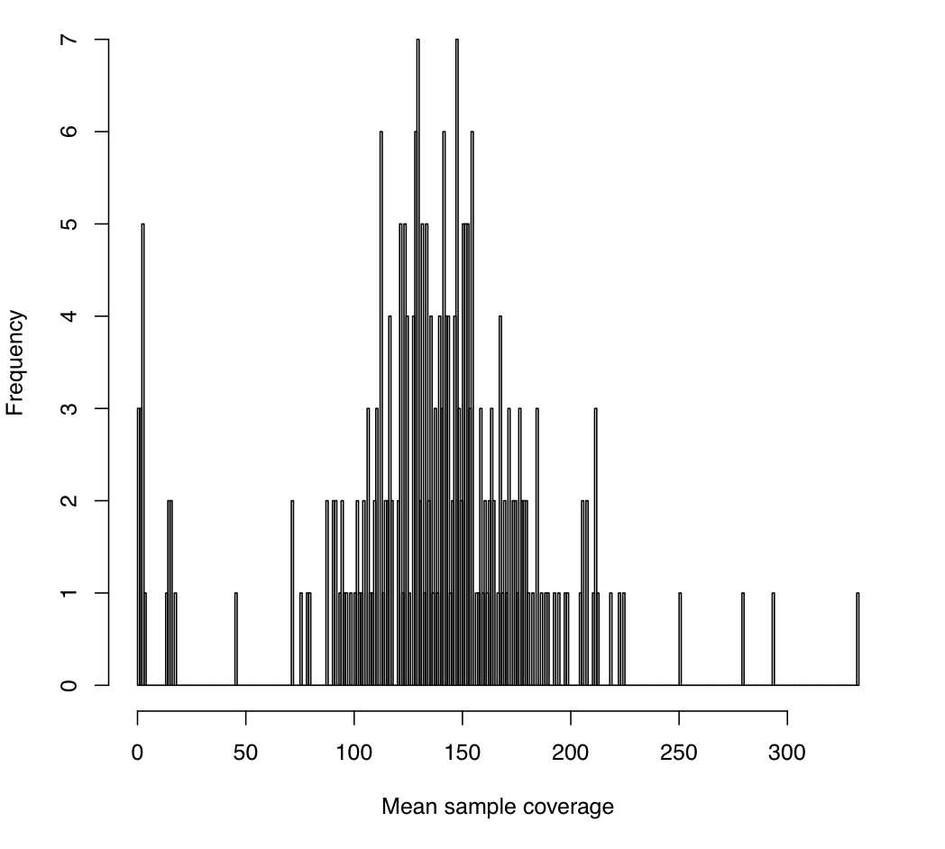
This image gives the sample-wide distribution of exome-wide coverage, where each per-sample coverage value is the mean of the coverage values calculated for each exome target (which itself is the mean coverage at all of its bases in that particular sample). In this experiment, we sequenced each sample to a mean coverage of 150x, so that we expect a typical sample to indeed have 150 reads covering an average base in an average exome target.
And, you'll also similarly get: mean_target_coverage.pdf
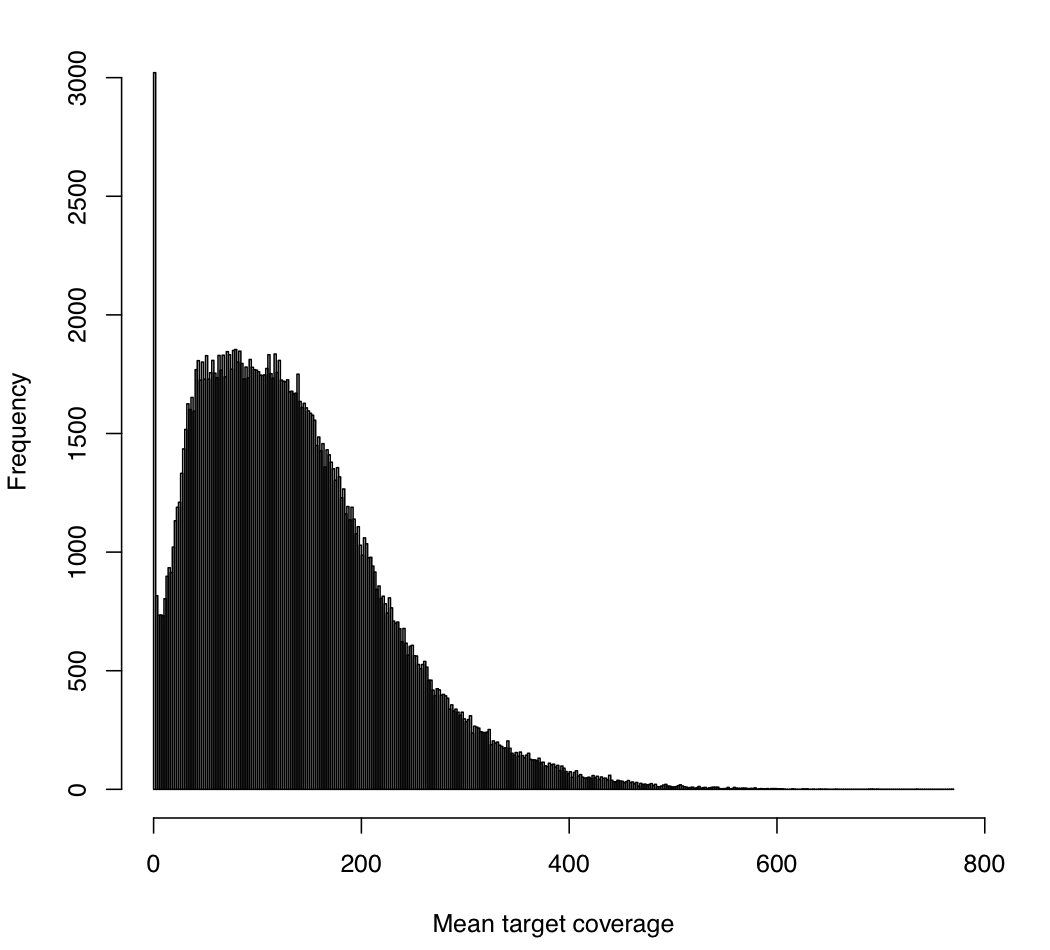
This analogously gives the target-wide distribution of coverage (over all samples). That is, each per-target coverage value is the mean of the per-sample coverage values at that target (where again, this is the mean coverage at all of its bases in that sample). As above, since our goal was to have 150x coverage exome-wide, we'd expect each target to have around 150x coverage, but we see here that there is high variability in target coverage. For example, some targets have as much 400x coverage (averaged over all samples), and we also see a non-trivial number of targets that have 0 coverage for all samples (e.g., targets where capture has presumably failed).
Next, we consider the principal component analysis (PCA) normalization stage. We compare each of the principal components to known sample and target features: PC_correlations.pdf
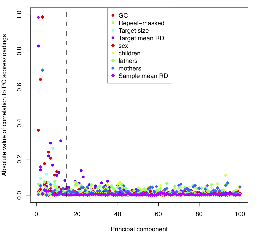
The dotted line (at PC = 15) indicates that XHMM automatically removed the 1st 15 components based on their significant relative variance. Now, in this plot we consider known sample and target features (that XHMM did not incorporate in its decision to remove them). We see that these 1st 15 PC tend to show correlation with various target features (colored circles) such as GC content and the mean depth of sequencing coverage at that target, and also with various sample features (colored diamonds) such as gender and mean depth of sequencing for that sample. On the other hand, there is a marked change in quality of the PC after the 1st 15 or so, with a sudden drop-off in the levels of correlation with genome-wide and batch effects expected to strongly bias the read depth of coverage.
Related to this is the "scree" plot for the PCA, showing the standard deviation of the depth data independently ascribed to each of the principal components: PC_stddev.pdf
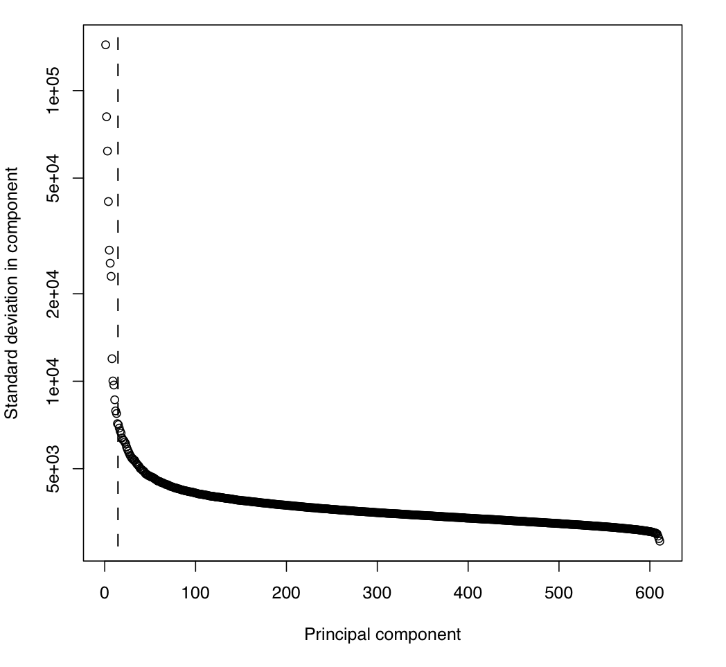
This case is typical, where we see that the cut-off automatically detected by XHMM corresponds to a significant drop in the variance (an "elbow" in the curve). Note the log scale of the y axis.
In the output directory, the "PC" sub-directory is created, which contains plots of the read depth data projected into each of the principal components: PC/PC.*.png
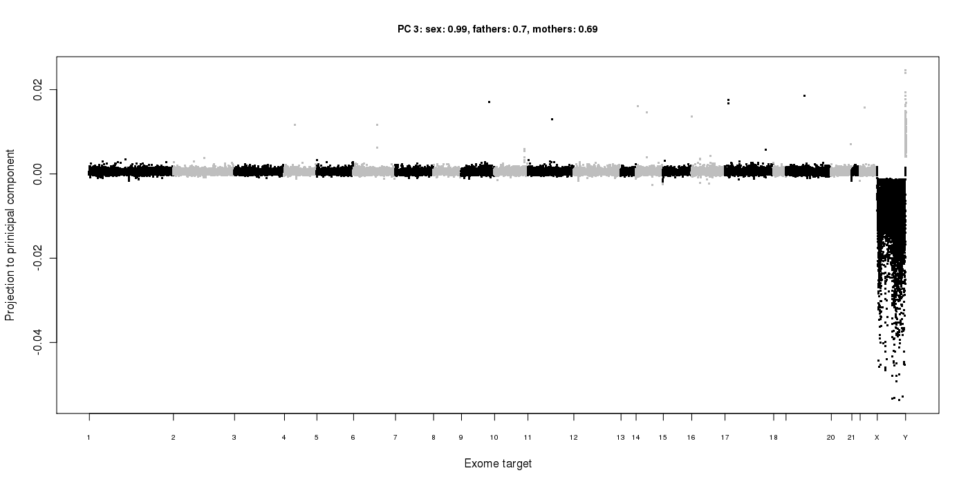
This principal component (the 3rd one, in this case) has found the variance in read depth due to gender differences, with males having lower coverage on the X chromosome and higher coverage on the Y. Therefore, the loadings for this component have a correlation of 0.99 with the gender of the samples.
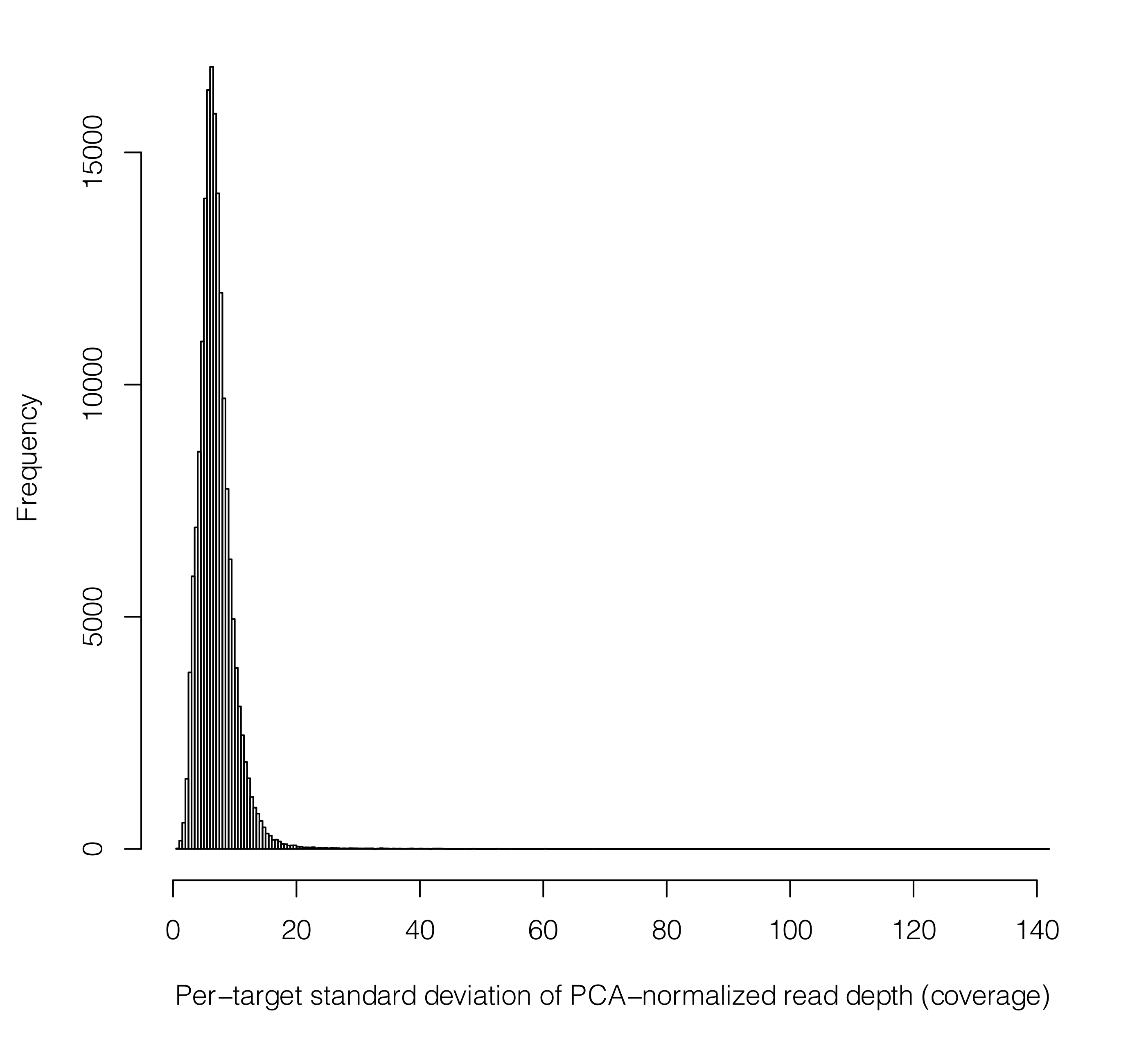
Next, before z-scores are calculated and the HMM is run to call CNV for each sample, we perform a final filtering step. Here, we remove any targets that have "very scattered" read depth distributions post normalization. These can be thought of as targets for which the normalization may have failed, and it is better to remove such strong effects (still likely to be artifacts) to prevent them from drowning out other more subtle signals. To do this, we remove any targets with large standard deviations of their post-normalization read depths across all samples. As a (proto-typical) example, we see here that the small fraction of targets with standard deviations any larger than the 30 to 50 range should be removed (in this case, for a scenario of ~ 100x mean sequencing coverage). This plot will be output to: per_target_sd.pdf
Lastly, in the "plot_CNV" sub-directory, a plot is made focusing on each CNV called in each individual (as found in the .xcnv file): plot_CNV/sample_*.png
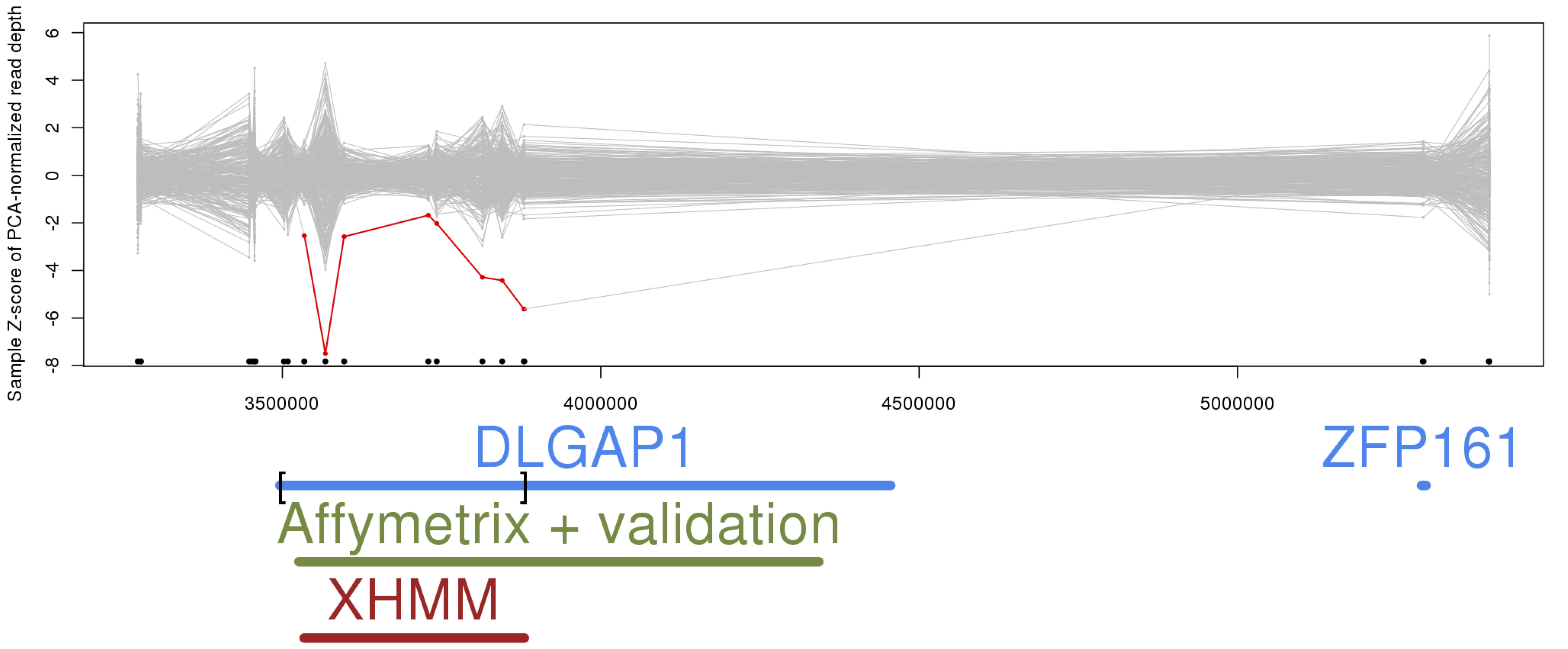
The example above shows a de novo deletion called by XHMM (in red) spanning the DLGAP1 gene (discussed in this study and previously validated in this study).
In general, these plots show each sample's read depths at each of the targets in focus, which are connected by gray lines. If the sample has a called deletion, then it's colored in red, and duplications in green. Gene names are added below to annotate the genomic region.
Also, it's important to note that, by default, a plot is generated for EACH CNV called by XHMM, without considering its quality score or frequency in the sample. As for many analyses, it is incumbent upon the researcher to consider the metrics and properties of the data set as a whole before considering any one particular CNV call. That is, here we recommend filtering on both the SQ quality threshold (the "Q_SOME" column in the .xcnv file) and filtering on sample-wide frequency to obtain a high-quality call set. See the publications for details.
A full list of XHMM command-line options:
The list below can be obtained by running:
./xhmm -h


  -h, --help                    Print help and exit
      --detailed-help           Print help, including all details and hidden
                                  options, and exit
      --full-help               Print help, including hidden options, and exit
  -V, --version                 Print version and exit

*******************************************************************
Options for modes: 'prepareTargets', 'genotype':
  -F, --referenceFASTA=STRING   Reference FASTA file (MUST have .fai index
                                  file)

*******************************************************************
Options for modes: 'matrix', 'PCA', 'normalize', 'discover', 'genotype':
  -r, --readDepths=STRING       Matrix of *input* read-depths, where rows
                                  (samples) and columns (targets) are labeled
                                  (default=`-')
*******************************************************************

 Mode: prepareTargets
  Sort all target intervals, merge overlapping ones, and print the resulting
  interval list
  -S, --prepareTargets
      --targets=STRING          Input targets lists
      --mergedTargets=STRING    Output targets list  (default=`-')

 Mode: mergeGATKdepths
  Merge the output from GATK into a single read depth matrix of samples (rows)
  by targets (columns)
  -A, --mergeGATKdepths
      --GATKdepths=STRING       GATK sample_interval_summary output file(s) to
                                  be merged [must have *IDENTICAL* target
                                  lists]
      --GATKdepthsList=STRING   A file containing a list of GATK
                                  sample_interval_summary output files to be
                                  merged [must have *IDENTICAL* target lists]
      --sampleIDmap=STRING      File containing mappings of sample names to new
                                  sample names (in columns designated by
                                  fromID, toID)
      --fromID=INT              Column number of OLD sample IDs to map
                                  (default=`1')
      --toID=INT                Column number of NEW sample IDs to map
                                  (default=`2')

 Mode: matrix
  Process (filter, center, etc.) a read depth matrix and output the resulting
  matrix.  Note that first all excluded samples and targets are removed.  And,
  sample statistics used for filtering are calculated only *after* filtering
  out relevant targets.
  -M, --matrix
      --excludeTargets=STRING   File(s) of targets to exclude
      --excludeChromosomeTargets=STRING
                                Target chromosome(s) to exclude
      --excludeSamples=STRING   File(s) of samples to exclude
      --minTargetSize=INT       Minimum size of target (in bp) to process
                                  (default=`0')
      --maxTargetSize=INT       Maximum size of target (in bp) to process
      --minMeanTargetRD=DOUBLE  Minimum per-target mean RD to require for
                                  target to be processed
      --maxMeanTargetRD=DOUBLE  Maximum per-target mean RD to require for
                                  target to be processed
      --minSdTargetRD=DOUBLE    Minimum per-target standard deviation of RD to
                                  require for target to be processed
                                  (default=`0')
      --maxSdTargetRD=DOUBLE    Maximum per-target standard deviation of RD to
                                  require for target to be processed
      --minMeanSampleRD=DOUBLE  Minimum per-sample mean RD to require for
                                  sample to be processed
      --maxMeanSampleRD=DOUBLE  Maximum per-sample mean RD to require for
                                  sample to be processed
      --minSdSampleRD=DOUBLE    Minimum per-sample standard deviation of RD to
                                  require for sample to be processed
                                  (default=`0')
      --maxSdSampleRD=DOUBLE    Maximum per-sample standard deviation of RD to
                                  require for sample to be processed
      --centerData              Output sample- or target- centered read-depth
                                  matrix (as per --centerType)  (default=off)
      --centerType=ENUM         If --centerData given, then center the data
                                  around this dimension  (possible
                                  values="target", "sample")
      --zScoreData              If --centerData given, then additionally
                                  normalize by standard deviation (outputting
                                  z-scores)  (default=off)
      --outputExcludedTargets=STRING
                                File in which to output targets excluded by
                                  some criterion
      --outputExcludedSamples=STRING
                                File in which to output samples excluded by
                                  some criterion

Options for modes: 'mergeGATKdepths', 'matrix':
  -o, --outputMatrix=STRING     Read-depth matrix output file  (default=`-')
*******************************************************************

 Mode: PCA
  Run PCA to create normalization factors for read depth matrix
  -P, --PCA                     Matrix is read from --readDepths argument;
                                  normalization factors sent to --PCAfiles
                                  argument

 Mode: normalize
  Apply PCA factors in order to normalize read depth matrix
  -N, --normalize               Matrix is read from --readDepths argument;
                                  normalization factors read from --PCAfiles
                                  argument
  -n, --normalizeOutput=STRING  Normalized read-depth matrix output file
                                  (default=`-')
      --PCnormalizeMethod=ENUM  Method to choose which prinicipal components
                                  are removed for data normalization  (possible
                                  values="numPCtoRemove", "PVE_mean",
                                  "PVE_contrib" default=`PVE_mean')
      --numPCtoRemove=INT       Number of highest principal components to
                                  filter out  (default=`20')
      --PVE_mean_factor=DOUBLE  Remove all principal components that
                                  individually explain more variance than this
                                  factor times the average (in the original
                                  PCA-ed data)  (default=`0.7')
      --PVE_contrib=DOUBLE      Remove the smallest number of principal
                                  components that explain this percent of the
                                  variance (in the original PCA-ed data)
                                  (default=`50')

Options for modes: 'PCA', 'normalize':
      --PCAfiles=STRING         Base file name for 'PCA' *output*, and
                                  'normalize' *input*
*******************************************************************

 Mode: discover
  Discover CNVs from normalized read depth matrix
  -D, --discover                Matrix is read from --readDepths argument
  -c, --xcnv=STRING             CNV output file  (default=`-')
  -t, --discoverSomeQualThresh=DOUBLE
                                Quality threshold for discovering a CNV in a
                                  sample  (default=`30')
  -s, --posteriorFiles=STRING   Base file name for posterior probabilities
                                  output files; if not given, and --xcnv is not
                                  '-', this will default to --xcnv argument

 Mode: genotype
  Genotype list of CNVs from normalized read depth matrix
  -G, --genotype                Matrix is read from --readDepths argument
  -g, --gxcnv=STRING            xhmm CNV input file to genotype in 'readDepths'
                                  sample
  -v, --vcf=STRING              Genotyped CNV output VCF file  (default=`-')
      --subsegments             In addition to genotyping the intervals
                                  specified in gxcnv, genotype all sub-segments
                                  of these intervals (with
                                  maxTargetsInSubsegment or fewer targets)
                                  (default=off)
      --maxTargetsInSubsegment=INT
                                When genotyping sub-segments of input
                                  intervals, only consider sub-segments
                                  consisting of this number of targets or fewer
                                   (default=`30')
  -T, --genotypeQualThresholdWhenNoExact=DOUBLE
                                Quality threshold for calling a genotype, used
                                  *ONLY* when 'gxcnv' does not contain the
                                  'Q_EXACT' field for the interval being
                                  genotyped  (default=`20')

Options for modes: 'discover', 'genotype', 'transition', 'printHMM':
  -p, --paramFile=STRING        (Initial) model parameters file

Options for modes: 'discover', 'genotype':
  -m, --maxNormalizedReadDepthVal=DOUBLE
                                Value at which to cap the absolute value of
                                  *normalized* input read depth values
                                  ('readDepths')  (default=`10')
  -q, --maxQualScore=DOUBLE     Value at which to cap the calculated quality
                                  scores  (default=`99')
  -e, --scorePrecision=INT      Decimal precision of quality scores
                                  (default=`0')
  -a, --aux_xcnv=STRING         Auxiliary CNV output file (may be VERY LARGE in
                                  'genotype' mode)
  -u, --auxUpstreamPrintTargs=INT
                                Number of targets to print upstream of CNV in
                                  'auxOutput' file  (default=`2')
  -w, --auxDownstreamPrintTargs=INT
                                Number of targets to print downstream of CNV in
                                  'auxOutput' file  (default=`2')
  -R, --origReadDepths=STRING   Matrix of unnormalized read-depths to use for
                                  CNV annotation, where rows (samples) and
                                  columns (targets) are labeled
*******************************************************************

 Mode: printHMM
  Print HMM model parameters and exit
      --printHMM

 Mode: transition
  Print HMM transition matrix for user-requested genomic distances
      --transition