PLINK offers a simple but potentially powerful approach to population stratification, that can use whole genome SNP data (the number of individuals is a greater determinant of how long it will take to run). We use complete linkage agglomerative clustering, based on pairwise identity-by-state (IBS) distance, but with some modifications to the clustering process: restrictions based on a significance test for whether two individuals belong to the same population (i.e. do not merge clusters that contain significantly different individuals) , a phenotype criterion (i.e. all pairs must contain at least one case and one control) and cluster size restrictions (i.e. such that, with a cluster size of 2, for example, the subsequent association test would implicitly match every case with its nearest control, as long as the case and control do not show evidence of belonging to different populations). In addition, external matching criteria can be specified, to match on age and sex, for example, as well as genetic information. Any evidence of population substructure (from this or any other analysis) can be incorporated in subsequent association tests via the specification of clusters.

All these analyses require genome-wide coverage of autosomal SNPs!

IBS clustering

To perform complete linkage clustering of individuals on the basis of autosomal genome-wide SNP data, the basic command is:

plink --file mydata --cluster

which generates four output files:

     plink.cluster0
     plink.cluster1
     plink.cluster2
     plink.cluster3

that contain similar information but in different formats. The

The *.cluster0 file contains some information on the clustering process. This file can be safely ignored by most users.

The *.cluster1 file contains information on the final solution, listed by cluster: e.g. for 4 individuals with the following Family and Individual IDs

we see 3 clusters, one line of output per cluster:

     0   A_1
     1   B_1 C_1
     2   D_1

(note how family and individuals IDs are concatenated with the underscore character in the output)

The *.cluster2 file contains the same information but listed one line per individual: the three columns are family ID, individual ID and assigned cluster:

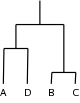
The *.cluster3 file is in the same format as cluster2 (one line per individual) but contains all solutions (i.e. every step of the clustering from moving from N clusters each of 1 individual (leftmost column after family and individual ID) to 1 cluster (labelled 0) containing all N individuals (the final, rightmost column): also shown is the dendrogram this represents: e.g.

     A 1 0 0 0 0
     B 1 1 1 1 0
     C 1 2 1 1 0
     D 1 3 2 0 0

NOTE If any constraints have been placed upon the clustering, then solutions represented in the *.cluster3 file may not go as far as 1 cluster with all N individuals: in this case, the file *.cluster2 will contain the final solution (i.e. as far as the clustering could go before running up against constraints, e.g. based on maximum cluster size, etc).

HINT! In large samples, cluster analyses can be very slow. Often the most time consuming step is calculating the pairwise IBS metrics: these only need to be calculated once however, even if you want to run the cluster analysis multiple times (e.g. with different constraints). This is achieved with the --read-genome option, assuming you have previously run the --genome command. It is a good idea to not impose a threshold of the --genome output in this case. For example:

plink --bfile mydata --genome --out mydata

followed by multiple clustering commands (see below for descriptions of the cluster constraint parameters used here)

plink --bfile mydata --read-genome mydata.genome --cluster --ppc 0.01

and

plink --bfile mydata --read-genome mydata.genome --cluster --mc 2 --ibm 0.01

etc.

ADVANCED HINT! In very large samples, cluster analyses can be very, very slow. When calculating the plink.genome file (as described above), if you have access to a cluster of computers for parallel computing, you can use the following approach to greatly reduce the time this step takes. In this case, we will assume you are familiar with and using a Linux operating system, and that the bsub prefix is used to send a job to the cluster -- obviously, change the script below as appropriate. This uses the --genome-lists option to calculate IBS statistics for only a subset of the sample at a time. If the binary fileset is data.* then create multiple lists of, for example, 100 individuals per list

     gawk '{print $1,$2}' data.fam | split -d -a 3 -l 100 - tmp.list

If this creates, for example, 39 separate files (labelled 0 to 38), then run these in all unqiue pairwise combinations in parallel with something like the following script: (i.e. edit the first line as appropriate)

     let i=0 a=38
     let j=0

     while [ $i -le $a ]
     do
      while [ $j -le $a ]
      do

         bsub -o /dev/null -e /dev/null ./plink --bfile data \
                 --read-freq plink.frq \
                 --genome \
                 --genome-lists tmp.list`printf "%03i\n" $i` \
                                tmp.list`printf "%03i\n" $j` \
                 --out data.sub.$i.$j

      let j=$j+1
      done

      let i=$i+1
      let j=$i

     done

NOTE If you use this approach to calculate the IBD probabilities, then you should first perform --freq on the whole dataset, then add the line --read-freq plink.frq (obviously replacing the filename with your file) to make sure that everybody has the sample frequencies used in the IBD calculations.

The finally, concatenate these individual files back into one (multiple header rows will be ignored, as FID is a reserved ID):

     cat data.sub*genome > data.genome
     rm tmp.list*
     rm data.sub.*

HINT As of v1.07, PLINK can directly read and write compressed .genome files. This is the preferred mode for large samples. For example

plink --bfile mydata --Z-genome --out mydata

creates a file

     mydata.genome.gz

This can be handled with the gunzip tool, or zcat, zgrep, zless, etc. PLINK can read such a file with --read-genome. Whether or not the file is compressed will be automatically detected (indicated by a .gz extension)

plink --bfile mydata --read-genome mydata.genome.gz ...

Note that several compressed files can be directly concatenated with the Unix cat command, without being decompressed first:

cat mydata-1.genome.gz mydata-2.genome.gz mydata-3.genome.gz > alldata.genome.gz

plink --bfile example --read-genome alldata.genome.gz ...

Permutation test for between group IBS differences

Given that pairwise IBS distances between all individuals have been calculated, we can asked whether or not there are group differences in this metric, with respect to a binary phenotype. The command

./plink --bfile mydata --ibs-test

or, if an appropriate plink.genome file has already been created,

./plink --bfile mydata --read-genome plink.genome --ibs-test

will permute case/control label, and then recalculate several between-group metrics based on average IBS within that group. This command uses a fixed 10,000 permutations.

All results are written to the LOG file. First, the observed means and standard deviation of each of the 3 groups (case/control, case/case and control/control, in that order) will be displayed: e.g.

     Between-group IBS (mean, SD) = 0.782377, 0.00203459
     In-group (2) IBS (mean, SD) = 0.782101, 0.00232296
     In-group (1) IBS (mean, SD) = 0.78273, 0.00170816

Then 12 separate tests are presented, which have self-explanatory names. If the label does not explicitly mention a comparison pair-type, it implies that the first pair type is being compared to the other two pair-types.

      T1: Case/control less similar                     p = 0.97674
      T2: Case/control more similar                     p = 0.0232698

      T3: Case/case less similar than control/control   p = 0.00285997
      T4: Case/case more similar than control/control   p = 0.99715

      T5: Case/case less similar                        p = 0.00430996
      T6: Case/case more similar                        p = 0.9957

      T7: Control/control less similar                  p = 0.99883
      T8: Control/control more similar                  p = 0.00117999

      T9: Case/case less similar than case/control      p = 0.00726993
     T10: Case/case more similar than case/control      p = 0.99274

     T11: Control/control less similar than case/control p = 1
     T12: Control/control more similar than case/control p = 9.9999e-06

For the purpose of stratification effects between cases and conrtols, the test T1 is probably most appropriate, as it directly asks whether or not, on average, an individual is less similar to another phenotypically-discordant individual than would be expected by chance (i.e. if we randomized phenotype labels). That is, to the extent that cases and controls are from two separate populations, you would expect pairs within a phenotype group to be more similar than pairs across the two groups, i.e. T1. Of course, the opposite could also be true (tested by T2), which would probably represent certain ascertainment procedures (i.e. taking this to an extreme, imagine a discordant sibling pair design: case/control pairs would on average be more similar than case/case and control/control pairs).

The other tests are provided for completeness and give a more general description of the variability between and within each group. The general pattern shown above would suggest that there is relatively more variability within the case sample than the control sample. Bear in mind when interpreting the empirical p-values that the relative sizes of case and control samples will have an impact on the exact p-value (i.e. these significance tests should not be taken to directly represent the magnitude of differences between groups).

Note This test assumes that individuals have a disease phenotype; obviously, one could swap in other labels (e.g. site of collection) via the --pheno command, as long as they are dichotomous.

Constraints on clustering

This section describes the extra constraints that can be placed on the clustering procedure, specified via other options in addition to the --cluster option. As further described in the association analysis and permutation sections, these options can be used to set up various types of analyses that control for potential stratification in the sample.

1) Based on pairwise population concordance (PPC) test:
This is a simple significance test for whether two individuals belong to the same random-mating population. To only merge clusters that do not contain individuals differing at a certain p-value:

--ppc 0.0001

NOTE This command has been changed from --pmerge in older versions of PLINK (pre 0.99n).

This test is based on the observed binomial proportion of IBS 0 loci pairs to IBS 2 het/het pairs: counts of these two types should be in the ratio of 1:2 if the two individuals come from the same population. The significant p-value indicates fewer IBS2 het/het loci than expected (based on normal approximation to binomial). These tests are also given by the --genome command.

WARNING! Unlike the basic IBS clustering, which places no restrictions on the SNPs that can be used in the analysis, this test assumes that the SNPs used are in linkage equilibrium. By default, this test will only count an 'informative' SNP pair (i.e. one that, for a particular pair of individuals, has two of each allele) as either an IBS 0 or IBS 2 count for this test (the HOMHOM and HETHET counts from the --genome option) if it is more than 500 kb more the previous informative pair of SNPs, for that particular pair of individuals. This gap parameter can be changed with the option

--ppc-gap 100

which would, in this case, reduce that gap to 100kb. (Note: all SNPs will still be used to calculate the main IBS distance metric, upon which the clustering is based).

HINT Also, this test is susceptible to non-random missingness in genotypes, particularly if heterozygotes are more likely to be dropped. It is therefore good practice to set the --geno very low for this analysis, i.e. so only SNPs with virtually complete genotyping are included.

2) Based on phenotype:
To ensure that every cluster has at least one case and one control:

--cc

3) Based on maximum cluster size:
To set the maximum cluster size to a certain value, e.g. 2:

--mc 2

Alternatively, to specify a maximum number of cases and a maximum number of controls per cluster, use the option:

--mcc 1 3

which, in this case, specifies that each cluster can have up to 1 case and 3 controls. Note the different syntax: -mcc as opposed to --mc. Using this in conjunction with the --cc constraint (that ensures at least 1 case and 1 control per cluster) this is an easy way to achieve a certain matching scheme, say 1 case to 3 controls, or 2 cases to 2 controls, etc.

4) Based on fixed number of clusters:
To request that the clustering process stops at a certain fixed number of clusters, for example, a 2 cluster solution, use:

--K 2

Note If other clustering constraints are in place, it is possible that clustering may stop before reaching the specified number of clusters with the --K option; if other constraints are specified, you can think of this as stating the minimum number of clusters possible.

5) Based on pattern of missing genotype data:
To only cluster individuals with sufficiently similar profiles of missing genotype data (genome-wide) use the option:

--ibm 0.02

which would only match people if they are discordantly missing (i.e. one person is missing a particular SNP but the other person is not) for 2 percent of the genome or less. Another way to incorporate missingness would be by defining overall call rate per individual as an external quantitative matching criteria (see below); this approach is preferrable however (as it does not match just on average rate, but also on whether it tends to be the same SNPs that are missing).

6) Based on user-specified external matching criteria:
To use external matching criteria: for categorical matching criteria, use the option:

--match mydata.match

where the file mydata.match contains the following columns: family and individual ID and the one or more matching variables, one row per person:

     Family ID
     Individual ID
     Matching criteria 1
     Matching criteria 2
     ...
     Matching criteria N

The default behavior is that only individuals with the same matching criteria across all the measures will be paired to make clusters. For example, if the file were:

     F1 I1   1  1  1
     F2 I2   1  2  1
     F3 I3   2  2  2
     F4 I4   1  2  1
     F5 I5   1  1  1
     ...

then only F1/I1 and F5/I5 could be paired; also F2/I2 and F4/I4 could be paired. No other combinations of pairings would be possible. Therefore, no cluster would ever be formed that contained both individuals F1/I1 and F2/I2, for example.

One application of this option would be to ensure that individuals are sex-matched, or matched on some relevant environmental exposure, in addition to the genetic IBS matching.

It is possible to adjust the default behaviour to consider two individuals as potentially 'pairable' is they differ on a particular categorical criteria. This is achieved with the optional command:

--match-type mydata.bt

where mydata.bt is the name of a file that contains a series of 0s and 1s (or "-" and "+" characters), whitespace delimited, that indicate whether a criteria should be a "postive match" (i.e. two individuals are potentially pairable only if they have the same values for this variable) or a "negative match" (i.e. two individuals are potentially pairable only if they have different values for this variable). In the above example, if the file mydata.bt were

+ - +

then the following pairs are potentially pairable:

     F1/I1 and F2/I2
     F1/I1 and F4/I4
     F5/I5 and F2/I2
     F5/I5 and F4/I4

i.e. F1/I1 can no longer be paired with F5/I5 because they have the same value for the second matching variable, which is now a negative match criteria.

Note In this example, the matching variables only took two values: in practice, one can have any number of categories per matching variable.

Note Missing variables can be specified for matching variables -- this means that the criteria will be ignored. As all pairs start out as potentially pairable, this means that missing matching criteria data will never be used to make a pair unpairable.

A second form a matching is based on quantitative traits -- in this case, a maximum difference threshold is specified for each measure, such that individuals will not be matched if they differ beyond the threshold on the quantitative traits. This is achieved by the following options:

--qmatch mydata.match --qt mydata.qt

Note that a second --qt option is necessary as well as the --qmatch option. The --qt specifies a file that contains the thresholds, e.g. for 3 external quantitative criteria, this should contain 3 values:

    5
    0.333
    120

The --qmatch should then contain the same number of quantitative matching criteria per person (again, one row per person):

     F1 I1   27  -0.23   1003
     F2 I2   34   2.22   1038
     F3 I3   45   1.99    987
     F4 I4   19  -9      2374
     F5 I5   18  -0.45    996
     ...

In this case, for example, for the first measure only F4/I4 and F5/I5 are pairable, as |19-18| is not more than 5. This measure might represent age, for example. This pair is not matchable on the basis on the third metric, however, as |2374-996| > 120. As such, no pairs could be formed between any of these five individuals, in this particular case. Note that individual is actually missing (default --missing-phenotype value is -9) for the second criterion: see below for a description of how missing data are handled in this context.

The .match and .qmatch files do not need to contain all individuals and do not need to be in the same order as the original PED files. Any individuals in these files who are not in the original files will be ignored.

Missing phenotypes are simply ignored (i.e. two individuals would not be called non-matching if either one or both had missing matching criteria). That is, the default for two individuals is that they are pairable -- only non-missing, non-matching external criteria (as well as the p-value test based on genetic data, described above) will make a pair unpairable.

IBS similarity matrix

For the N individuals in a sample, to create a N x N matrix of genome-wide average IBS pairwise identities:

plink --file mydata --cluster --matrix

creates the file

     plink.mibs

which contains a square, symmetric matrix of the IBS distances for all pairs of individuals. These values range, in theory, from 0 to 1. In practice, one would never expect to observe values near 0 -- even completely unrelated individuals would be expected to share a very large proportion of the genome identical by state by chance alone (i.e. as opposed to identity by descent). A value of 1 would indicate a MZ twin pair, or a sample duplication. More details on pairwise relatedness can be obtained by using the --genome command.

The default behavior of --matrix to to output similarities (proportions of alleles IBS). To generate a distance matrix (1-IBS) then use the command

plink --file mydata --cluster --distance-matrix

instead. This will generate a file

     plink.mdist

HINT See the FAQ page for instructions on using using R to visualise these results; alternatively, use the --mds-plot option described below.

NOTE In versions prior to v1.00, there is no --distance-matrix command and --matrix outputs a file called plink.mdist rather than plink.mibs -- these are still similarities, not distances.

Multidimensional scaling plots

To perform multidimensional scaling analysis on the N x N matrix of genome-wide IBS pairwise distances, use the --mds-plot option in conjunction with --cluster. This command takes a single parameter, the number of dimensions to be extracted. For example, assuming we have already calculated the plink.genome file,

plink --file mydata --read-genome plink.genome --cluster --mds-plot 4

creates the file

     plink.mds

which contains one row per individual, with the fields

     FID    Family ID
     IID    Individual ID
     SOL    Assigned solution code (from --cluster)
     C1     Position on first dimension
     C2     Position on second dimension
     C3     Position on third dimension
     C4     Position on fourth dimension

Plotting the C1 values against C2, for example, will give a scatter plot in which each point is an individual; the two axes correspond to a reduced representation of the data in two dimensions, which can be useful for identifying any clustering. Standard classical (metric) multidimensional scaling is used.

Instead of using each individual as the unit of analysis, you can make each point a cluster from the final solution (as determined by --cluster along with whatever constraints were imposed) and the distances between clusters are the average distances of all individuals in those clusters. Use the --mds-cluster flag (as well as --cluster --mds-plot K) for this.

Speeding up MDS plots: 1. Use the LAPACK library

If you compile PLINK to use the LAPACK library to perform the SVD used in the MDS analysis, this can significantly speed things up. This involves, LAPACK being available on your system, and compiling PLINK from source, with a flag set to use that library. Otherwise, no changes are made to the command: the same --mds-plot command is used. A line will be written the LOG file file indicating that the LAPACK library was used

    Writing MDS solution to [ v2.mds ]
    MDS plot of individuals (not clusters)
    Using LAPACK SVD library function...

NOTE This should give similar results, although it is possible that the sign of various components might be flipped: this is expected and of no concern.

See these notes for help on how to compile PLINK to use LAPACK. Please note that I cannot provide support on how to compile LAPACK on your specific system. LAPACK is a set of FORTRAN programs (and requires gfortran to compile) -- ask your IT people for help if needed.

Speeding up MDS plots: 2. pre-cluster individuals

With large samples (over 10,000 individuals say) MDS plots can become very slow. One possible way to speed things up slightly is to first group individuals into groups of fairly similar individuals, and then perform the MDS analysis on the groups rather than the individuals (i.e. based on the mean distances between groups). PLINK will output a file in which each individual in the same group has the identical MDS components therefore. To use this option, add --mds-cluster and --within, for example

plink --bfile mydata 
      --read-genome mydata.genome 
      --mds-plot 4
      --mds-cluster
      --within clst.cluster2

This would be appropriate, for example, if the clst.cluster2 file resulted from a prior cluster analysis (using --cluster) with a setting such as

     --mc 10

to create a fairly large number of small groups (max 10 per group). Obviously, --mds-cluster will not give sensible results if there are too few clusters, or if the clusters are too big.

Outlier detecion diagnostics

Sometimes it can be useful to detect a handful of individuals who do not cluster with an otherwise fairly homogeneous sample. It is possible to generate some metrics describing much of an 'outlier' an individual is with respect to the other individuals in that sample, based on the genome-wide IBS information, as decribed above.

For any one individual, we can rank order all other individuals on the basis of how similar (in IBS terms) they are to this particular proband individual. We can then ask, is the proband's closest neighbour significantly more distant to the proband than all other individuals' nearest neighbour is to them. In otherwords, from the distribution of 'nearest neighbour' scores, one for each individual, we can calculate a sample mean and variance and transform this measure into a Z score. If an individual has an extreme low Z score, say less than 4 standard deviation units, this would indicate that this individual is an outlier with respect to the rest of the sample (i.e. this individual's nearest neighbour is a lot less near than the average nearest neighbour). As well as performing this test with the nearest neighbour, we can also perform it with the distribution of second-closest neighbours for each individual; then third closest neighbours, etc. It might sometimes be more informative to look at these 'second-closest' and 'third-closest' measures, to detect, for instance, a pair of individuals who are very similar to each other, but very distant from the rest of the sample -- they would score normally on the 'first-closest' neighbour test, but not on the 'second-closest', 'third-closest' tests, etc. It might sometimes be informative to look at the whole distribution of these 'neighbour' metrics, going to 1st nearest to the Nth nearest.

Another metric which can be used to identify potential outliers is, for each individual, to calculate the proportion of binomial IBS tests (described in the constaints section above), for each individual, that showed a significant difference at the --ppc threshold.

The basic option is, for example:

plink --file data --cluster --neighbour 1 5

This command always takes two arguments, specifying, in this case, to consider from the 1st nearest neighbour to the 5th nearest neighbour; this option generates the output file:

     plink.nearest

which contains the fields:

     FID          Family ID
     IID          Individual ID
     NN	          Nearest neighbour level (see below)
     MIN_DST      IBS distance of nth nearest neighbour (see below)
     Z            MIN_DST converted to a Z score (see below)
     FID2         Family ID of the nth nearest neighbour
     IID2         Individual ID of the nth nearest neighbour
     PROP_DIFF    Proportion of significantly different others (see below)

Looking at some example output, in this case for two individuals from the Asian HapMap samples, measured on around 50K random SNPs, for nearest neighbours 1 to 5, we see:

   FID      IID     NN      MIN_DST            Z   FID2   IID2  PROP_DIFF
   JPT256     1      1       0.7422       0.8897   JPT265    1    0.01136
   JPT256     1      2        0.742        1.223   JPT236    1    0.01136
   JPT256     1      3       0.7408       0.6503   JPT261    1    0.01136
   JPT256     1      4       0.7405       0.7285   JPT250    1    0.01136
   JPT256     1      5       0.7402       0.6204   JPT269    1    0.01136

   JPT257     1      1       0.7368       -3.701   JPT242    1     0.9318
   JPT257     1      2       0.7364       -3.463   JPT238    1     0.9318
   JPT257     1      3       0.7359       -3.832   JPT244    1     0.9318
   JPT257     1      4       0.7356       -3.974   JPT245    1     0.9318
   JPT257     1      5       0.7353       -4.046   JPT228    1     0.9318

Here we clearly see that the individual coded as JPT257 seems to be an outlier, with these first five measures being around 4 standard deviations below the group mean. In contrast, individual JPT256 does not appear to be an outlier, as the Z scores are above the mean (greater than 0). Plotting the Z scores for the entire sample makes it clear that JPT257 is indeed an outlier, as does the result for the IBS test -- JPT257 is significant different from 93% of the rest of the sample (the threshold for the IBS test is set to be quite stringent here, 0.0005 -- this is changed with the --ppc option as described above). At this fairly strict level, the subtle differences between Japanese and Han Chinese individuals are not detected -- using a threshold at 0.05, for example, one would see that many individuals show greater than the expected 0.05 in the PROP_DIFF field, as it is now picking up this group difference.

This document last modified Wednesday, 25-Jan-2017 11:39:28 EST

Whole genome association analysis toolset

Population stratification