This page describes some basic file formats, convenience functions and analysis options for rare copy number variant (CNV) data. Support for common copy number polymorphisms (CNPs) is described here.

Copy number variants are represented as segments. These segments are essentially represented and analysed in a similar manner to how PLINK handles runs of homozygosity (defined by a start and stop site on a given chromosome). Allelic (i.e. basic SNP) information is not considered here: PLINK skips the usual procedure of reading in SNP genotype data.

Here we assume that some other software package such as the Birdsuite package has previously been used to make calls for either specific copy-number variable genotypes or to identify particular genomic regions in individuals that are deletions or duplications, based on the raw data. That is, PLINK only offers functions for downstream analysis of CNV data, not for identifying CNVs in the first place, i.e. similar to the distinction between SNP genotype calling versus the subsequent analysis of those calls.

In this section, we describe the basic format for rare CNV data; the steps involved in making a MAP file and loading the data. We consider ways to filter the CNV lists by type, genomic location or frequency. We describe options for relating CNVs to phenotype, either at the level of genome-wide burden or looking for specific associations. Finally, we detail the tools for producing reports of any genes intersected by CNVs and for displaying groups of overlapping CNVs.

Basic support for segmental CNV data

The basic command for reading a list of segmental CN variants is

  plink --cnv-list mydata.cnv
        --fam mydata.fam
        --map mydata.cnv.map

which can be abbreviated

plink --cfile mydata

(note that the map file must have the .cnv.map map extension). The CNV list file mydata.cnv has the format

     FID     Family ID
     IID     Individual ID
     CHR     Chromosome
     BP1     Start position (base-pair)
     BP2     End position (base-pair)
     TYPE    Type of variant, e.g. 0,1 or 3,4 copies
     SCORE   Confidence score associated with variant 
     SITES   Number of probes in the variant

Having a header row is optional; if the first line starts with FID it will be ignored.

Note The SCORE and SITES values are not used in any direct way, except potentially as variates to filter segments on, as described below. That is, the values of these do not fundamentally impact the way analysis is performed by PLINK itself (they might alter the meaning of the results of course, e.g. if including low-confidence calls into the analysis!). In other words, if whatever software was used to generate the CNV calls does not supply some conceptually similar values, it is okay to simply put dummy codes (e.g. all 0) in these two fields.

The first few lines of a small example file is shown here:

     FID    IID   CHR       BP1       BP2  TYPE   SCORE  SITE
     P1     P1      4  71338469  71459318     1      27     0
     P1     P1      5  31250352  32213542     1    34.2     0
     P1     P1      7  53205351  53481230     3    18.2     0
     P2     P2     11  86736484  87074601     1      22     0  
     P2     P2     14  47817280  47930190     4    55.1     0
     ...

The FAM file format is the first 6 fields of a PED file, described here; this file lists the sex, phenotype and founder status of each individual. The MAP file format is described here, although the next section how this can be automatically created using the --cnv-make-map command.

Creating MAP files for CNV data

Prior to any analysis, a dummy MAP first needs to be created (this step only needs to be performed once per CNV file). This PLINK-generated MAP file has dummy entries that correspond to the start and stop sites of all segments. This facilitates subsequent parsing and analysis of CNV data by PLINK. The --cnv-make-map command is used as follows:

plink --cnv-list mydata.cnv --cnv-make-map

which creates a file

     plink.cnv.map

which will look just like a standard MAP file but with dummy markers:

     1       p1-51593   0    51593
     1       p1-51598   0    51598
     1       p1-51666   0    51666
     1       p1-52282   0    52282
     1       p1-69061   0    69061
     ...

where the marker names start with the p prefix and contain chromosome and base-position information.

As an (unrealistic) example to illustrate how the mapping works, consider the following, with 3 segments, spanning "positions" 1 to 8, 4 to 12 and 16 to 23. In this case, 6 unqiue map positions would be created, the three start positions and the three stop positions.

        Base                1111111111222222
        Position   1234567890123456789012345  

        Marker #   1..2...3...4...5......6..
                   |  |   |   |   |      |
                              |   |      |
        Segments   *------*       |      |
                      *-------*             
                                  *------*

The new MAP file would then be

     1 p1-1   0  1
     1 p1-4   0  4
     1 p1-8   0  8
     1 p1-12  0  12
     1 p1-16  0  16
     1 p1-23  0  23

Given such a MAP file, these three segments would then be perfectly mapped to the corresponding markers (p1-1 to p1-8, p1-4 to p1-12 and p1-16 to p1-23). The created MAP file is then specified in subsequent segmental CNV analyses (using --cnv-list) with the standard --map command (or --cfile command).

Loading CNV data files

Once a suitable MAP file has been created, i.e. with dummy markers that correspond to the position of every start and stop site of all segments, use the --cnv-list command again to load in the CNV segment data. As mentioned above, in addition to the basic CNV file, a MAP (previously generated) and FAM file (continaing ID and phenotype information) also need to be specified. For example.

plink --map plink.cnv.map --fam mydata.fam --cnv-list mydata.cnv

Alternatively, if the MAP, FAM and CNV list files all have the same root, the command

plink --cfile study1

is equivalent, i.e. it implies the following files exist

     study1.cnv
     study1.cnv.map
     study1.fam

By default either command will simply load in the CNV data and produce a report in the LOG file, enumerating the number of CN states in the total dataset and any filtering processes applied. For example,

     Reading segment list (CNVs) from [ cnv1.list ]
     714 of 2203 mapped as valid segments
     1872 mapped to a person, of which 714 passed filters
        CopyN  Count
        0      46
        1      339
        3      200
        4      129
     Writing segment summary to [ plink.cnv.indiv ]

This indicates that of 2203 total segments (i.e. should correspond to number of lines in the cnv1.list file, allowing for any header) 1872 are mapped to a person in the dataset. In other words, some of the segments in cnv1.list are for individuals not in cnv1.fam. These are simply ignored; for example, these individuals might have been filtered out of the study for other reasons, e.g. QC based on standard SNP genotypes. Of these, 714 passed the further set of filters, as described below. As described below, segments can be filtered based on genomic location, frequency, size, quality score/number of sites and type (duplication or deletion).

It will also be reported in the LOG file if some of the segments do not map to a marker in the MAP file: if this is because you've used --chr or similar commands to restrict the portion of the data examined, you can safely ignore this line; otherwise, it might mean that the appropriate MAP file wasn't created (e.g. using --cnv-make-map) for that CNV file.

By default, PLINK will create a file that summarises per individual events (after any filtering has been applied), in a file named

     plink.cnv.indiv

which has the fields, one row per person, in the same order as the original FAM file:

     FID     Family ID
     IID     Individual ID
     PHE     Phenotype 
     NSEG    Number of segments that individual has
     KB      Total kilobase distance spanned by segments 
     KBAVG   Average segment size

PLINK will also create a file

     plink.cnv.summary

that represents a count of CNVs, in cases (AFF) and controls (UNAFF) that overlap each map position.

Checking for overlapping CNV calls (within the same individual)

As a sanity check of a CNV file: to check whether segments are overlapping for the same person (e.g. if a deletion and a duplication event had been specified for the same person in the same region, or if the same event is listed twice), use the option

plink --cfile mydata --cnv-check-no-overlap

If there is overlap, this writes a warning to the LOG, with the number of implicated events:

     Within-individual CNV overlap detected, involving 2 CNVs

and creates a file

     plink.cnv.overlap

that lists these offending segments, with the format:

     FID   Family ID
     IID   Individual ID
     CHR   Chromosome code
     BP1   Segment start (bp)
     BP2   Segment end (bp)

Filtering of CNV data based on CNV type

The segments read in can be filtered in a number of ways. First, one can specify to read in only either deletions (TYPE is less than 2) or duplications (TYPE is greater than 2), with the options,

   --cnv-del

and

   --cnv-dup

Segments can also be filtered based on a minimum size (kb), score or number of sites contributing with the following commands:

   --cnv-kb 50 
   --cnv-score 3
   --cnv-sites 5

The default minimum segment size is 20kb; none of the other filters have a default setting that would exclude anything. Also, corresponding maximum thresholds can be set:

   --cnv-max-kb 2000
   --cnv-max-score 10
   --cnv-max-sites 10

As mentioned above, the SCORE and SITES fields are not used for any other purpose in analysis, and so if you do not have this information, can can safely enter dummy information (e.g. a value of 1 for every CNV).

The set of individuals for whom segment data are based on can be modified with the standard --keep and --remove options, to exclude people from the analysis.

Filtering of CNV data based on genomic location

It is possible to extract a specific set of segments that overlap with one or more regions as specified in a file, e.g. that might contain the genomic co-ordinates for genes or segmental duplications, etc. Use the command

     --cnv-intersect regions.list

The file regions.list should be in the following format: one range per line, whitespace-separated:

     CHR     Chromosome code (1-22, X, Y, XY, MT, 0)
     BP1     Start of range, physical position in base units
     BP2     End of range, as above
     MISC    Any other fields after 3rd ignored

For example, if regions.list were

     2 30000000 35000000  REGION1
     2 60000000 62000000
     X 10000000 20000000  Linkage hotspot

then

plink --cfile mydata --cnv-intersect regions.list

would extract all segments in mydata.cnv that at least partially span these three regions (5Mb and 2Mb on chromosome 2 and 10Mb on chromosome X), ignoring the comments or gene names. A typical type of file used with --cnv-intersect will often be a list of genes (such as available in the resources page).

Alternatively, you can use

     --cnv-exclude regions.list

to filter out a specific set of segments, i.e. to remove any CNVs that overlap with one or more regions specified in the file regions.list.

Assuming the region file has consistent, unique names in the fourth field, the command

     --cnv-subset mylist.txt

takes a list of region names and extracts just these from the main --cnv-intersect, --cnv-exclude (or --cnv-count, as described below) list. e.g. if mylist.txt contained

     REGION1
     REGION2

and region.list where

     2 30000000 35000000  REGION1
     2 60000000 62000000  GENE22
     X 10000000 20000000  LinkageHotspot

then only the first region (chromosome 3, 30Mb to 35Mb, labelled REGION1) would be extracted, as REGION2 does not exist. The --cnv-subset command requires that the regions.list file has exactly four fields (i.e. always a unique region/gene name in the fourth field).

Defining overlap for partially overlapping CNVs and regions

The basic intersection or exclusion commands will select all segments that are at least partially in the specified region. Alternatively, one can select only segments that have at least X percent of them in the specified region, for example

     --cnv-overlap 0.50

would only include (--cnv-intersect), or exclude (--cnv-exclude), events that have at least 50% of their length spanned by the region.

There are two other variant forms of the overlap command, which change the denominator in calculating the proportion overlap:

     --cnv-union-overlap 0.50

which defines overlap as the ratio of the intersection and the union, also

     --cnv-region-overlap 0.50

which defines overlap as the ratio of the intersection and the length of the region (rather than the CNV). For example,


     ------|-----|---------------------   Region/gene
     ----------+++++++++++++++---------   CNV (duplication, +)

     ----------XXX---------------------   Intersection

     ----------XXXXXXXXXXXXXXX---------   Denominator for basic overlap
     ------XXXXXXXXXXXXXXXXXXX---------   Denominator for union overlap
     ------XXXXXXX---------------------   Denominator for region overlap

In this example, if we take each character to represent a standard length

     Default overlap = 3 / 15
     Union overlap = 3 / 19
     Region overlap = 3 / 7

This next example illustrates how the overlap statistics can then subsequently be used to include or exclude specific CNVs: if overlap threshold were set to 0.5, then only the first of therse two CNVs would be selected by --cnv-intersect

     ------|----------|----------------     
         
     --------OOOOOOOOOOXXX-------------   Selected

     ------------OOOOOOXXXXXXXXXXXXXX--   Not selected

The default setting is equivalent to setting --cnv-overlap 0 (i.e. more than 0% must overlap).

Finally, the command

     --cnv-disrupt

will select only CNVs that start or stop within a region specified in the region list (i.e. resulting in a partially deleted or duplicated gene or region). The normal overlap commands cannot be used in conjunction with the --cnv-disrupt defintion of whether or not a CNV overlaps a gene.

Filtering by chromosomal co-ordinates

In addition, the standard commands for filtering chromosomal positions are still applicable, for example

     --chr 5

     --chr 2 --from-mb 20 --to-mb 25

Note that for a CNV to be included when using these filters, both the start and stop site must fall within the prespecified range (i.e. a CNV spanning from 19 to 24Mb on chromosome 2 would not be included in the above example).

Filtering of CNV data based on frequency

It is also possible to exclude based on the frequency of CNVs at a particular position. There are two main approaches to this: by assigning frequencies for regions and then applying the same routines as for the range-intersection command described above, or alternatively by assigning each CNV a single, specific count.

These commands, and the differences between them, are described more fully on this page. As well as the two basic approaches described above, one can specify different degrees of overlap when calculating frequencies, which can alter the result of frequency filtering.

The key commands and some examples are given here. To remove segments that map to regions with more than 10 segments

     --cnv-freq-exclude-above 10

To remove any segments that only have at most 4 copies

     --cnv-freq-exclude-below 5

To remove any segments not in regions with exactly 5 copies

     --cnv-freq-exclude-exact 5

and correspondingly to include only segments in regions with exactly 5 copies

     --cnv-freq-include-exact 5

As with the earlier range intersection commands, the definition of intersection can be soft, specified with the --cnv-overlap option. In most cases here, one would probably want to allow for a soft filtering, e.g. with --cnv-overlap 0.5 for example.

For example, given the following segments, and counts below

        Segments   *------*       
                      *------------*             
                                  *------*
          Counts 001112222211111112211111100000
  Common regions      XXXXX       XX

then --cnv-freq-exclude-above 1 would remove all three segments if --cnv-overlap 0 (the default) were set. This is because each CNV has at least some part of it that intersects with a region that contains more than 1 CNV. However, if --cnv-overlap were instead set to 0.5, for example, then only the top segment would be removed (as the other two segments have more than 50% of their length outside of a region with more than 1 segment). If the overlap were set higher still, then in this example no CNVs would be removed by the command --cnv-freq-exclude-above 1.

NOTE Because multiple CNVs at the same region will not all exactly overlap, and may be spanned by distinct larger events, or contain smaller events, in other individuals, then requesting that you include only CNVs with exactly five copies for example (--cnv-freq-include-exact 5) does not mean that at all positions in the genome you will always see either 0 or 5 copies. Rather, the selection process works exactly as specified above. Please see this page for further details.

Alternative frequency filtering specification

The alternate approach is invoked with the command

     --cnv-freq-method2 0.5

where the value following it represents an overlap parameter (there is no need to specify the --cnv-overlap command directly when using --cnv-freq-method2). Based on this overlap, PLINK will assign a specific count to each CNV that represents the number of CNVs that overlap it (including itself) based on a union intersection overlap definition with the specified proportion parameter, between that CNV and all CNVs.

This approach is illustrated in the page, that gives more details on the frequency filtering commands including a comparison to the region-based approach to filtering, described above.

If the --cnv-freq-method2 command is used, then the other frequency filtering commands will use the CNV-based counts to include of exclude CNVs, for example

 plink --cfile mydata 
       --cnv-freq-method2 0.5
       --cnv-freq-exclude-above 10

If --cnv-write (see below) is specified with --cnv-freq-method2, then the additional command

     --cnv-write-freq

will add a field FREQ to the plink.cnv file generated that shows the frequency for each CNV. Also, the --cnv-seglist command (see below) can be modified with --cnv-write-freq (to report the frequency as a number at the start and stop of each CNV instead of the usual codes).

Miscellaneous commands frequency filtering commands

To keep only segments that are unique to either cases or to controls

     --cnv-unique

This can be used in conjunction with other frequency filter commands. To drop individuals from the file who do not have at least one segment after filtering, add the flag

     --cnv-drop-no-segment

This can make the plink.cnv.indiv summary files easy to browse, for example.

Burden analysis of segmental CNV data

To perform a set of global test of CNV burden in cases versus controls, add the

     --cnv-indiv-perm

option as well as

     --mperm 10000

for example (i.e. permutation is required). By default, this reports on four tests, which use these metrics to calculate burden in both cases and controls

     RATE    Number of segments
     PROP    Proportion of sample with one or more segment
     TOTKB   Total kb length spanned
     AVGKB   Average segment size

Tests are based (1-sided) on comparing these metrics in cases versus controls, evaluated by permutation.

If a list of regions is supplied in a file, e.g. gene.list and the command

     --cnv-count gene.list

then an extra test is added

     GRATE   Number of regions/genes spanned by CNVs
     GPROP   Number of CNVs with at least one gene
     GRICH   Number of regions/genes per total CNV kb

These tests respect all the normal filtering commands, with the exception that --cnv-intersect and --cnv-exclude cannot be used if --cnv-count is also being used.

The mean metrics in cases and controls are reported in the file

     plink.cnv.grp.summary

when the --cnv-indiv-perm command is used. For example: this gives the number of events (N) in cases and controls, the rate per person, the proportion of cases/controls to have at least one event, the total distance spanned per person and the average event size per person.

        TEST      GRP      AFF    UNAFF
           N      ALL      528      362
        RATE      ALL   0.1557   0.1138
        PROP      ALL   0.1309   0.1041
       TOTKB      ALL    290.8    265.4
       AVGKB      ALL    249.8    243.3

As usual, if the --within command is added and a cluster file specified, then any permutations are performed within cluster. In this case, the statistics displayed in the plink.cnv.grp.summary file are also split out by the strata as well as presented in total (as indicated by the GRP field).

Improved gene-set enrichment analysis for segmental CNV data

This test implements a geneset-enrichment method for CNV data described in Raychaudhuri et al, 2010. It is appropriate for either continuous or disease traits and allows for the inclusion of multiple other covariates and for empirical significance tests.

The following examples illustrate basic usage. If the file genes.dat contains the locations of all genes (i.e. as available from here and the file pathway.txt is a file of gene names forming the pathway to be tested for enrichment and the CNV data are in the files mycnv.cnv, mycnv.cnv.map and mycnv.fam as described above, then one can ask whether a) genes are enriched for CNVs, b) a subset of genes are enriched, relative to the whole genome, c) a subset of genes are enriched, relative to all genes. The latter form of the enrichment test might be desirable, for example, to determine whether any enrichment is general to all genes, or specific to a subset of genes.

To test for enrichment of genic CNVs:

  plink --cfile mycnv
        --cnv-count genes.dat
        --cnv-enrichment-test

Enrichment of pathway genes CNVs, relative to all CNVs

  plink --cfile mycnv
        --cnv-count genes.dat
        --cnv-subset pathway.txt
        --cnv-enrichment-test

To test for enrichment of pathway genes CNVs, relative to all genic CNVs

  plink --cfile mycnv
        --cnv-intersect genes.dat
        --cnv-write my-genic-cnv

  plink --cfile my-genic-cnv
        --cnv-count genes.dat
        --cnv-subset pathway.txt
        --cnv-enrichment-test

The usual modifiers (to define intersection differently, allow for a certain kb border around each gene, filter on CNV size, type or frequency, etc) are all available. Under all circumstances, 2-sided asymptotic p-values are returned. Alternatively, permutation testing can be applied and 1-sided empirical p-values are returned (positive enrichment in cases, based on estimated regression coefficient), by adding the flag:

  --mperm 10000

Association mapping with segmental CNV data

To perform a simple permutation-based test of association of segmental CNV data for case/control phenotypes, add the option

     --mperm 50000

to perform, for example, 50,000 null permutations to generate empirical p-values. T he results are saved in the file

     plink.cnv.summary.mperm

This is a standard empirical p-value file: EMP1 and EMP2 represent pointwise and genome-wide corrected p-values, respectively. Both tests are 1-sided by default.

You can consult the corresponding

     plink.cnv.summary

that is also generated for details of the association: this file has the fields

     CHR    Chromosome code
     SNP    SNP identifier (dummy SNP, see below)
     BP     Base-pair position
     AFF    Number of affected individuals with a segment at this position
     UNAFF  Number of unaffected individuals

To instead perform a 2-sided test (i.e. allowing that events might be more common in controls) add the flag

     --cnv-test-2sided

To perform an analysis in which the total number of events within a sliding window is compared between cases and controls (rather than the number overlapping a single position) add the flag

     --cnv-test-window 50

where the parameter is the kb window either side of the test position. As before, the association results are reported per marker, but now the counts indicate the total number of segments that overlap any of the 100kb window surrounding the test position (+/- 50kb), rather than just the test position itself. Significance is evaluated by permutation as before.

Association mapping with segmental CNV data: regional tests

To perform a test of association for CNVs in particular regions, use the command

./plink --cfile mydata --cnv-intersect glist-hg18 --cnv-test-region --mperm 10000

where glist-hg18 contains a list of genes (as available from the resources page. The output is written to

     plink.cnv.regional.summary

which has the fields

     CHR       Chromosome code
     REGION    Name of region
     BP1       Start position of region
     BP2       End position of region
     AFF       Number of case CNVs spanning region
     UNAFF     Number of control CNVs spanning region

and the permutation results are written to

     plink.cnv.regional.summary.mperm

which has the fields

     CHR     Chromosome code
     REGION  Name of region
     STAT    Statistic
     EMP1    Empirical p-value, per region
     EMP2    Empirical p-value, corrected for all tests

For example, the line

 CHR           REGION          BP1          BP2      AFF    UNAFF
   1           TTLL10      1079148      1143176        2        3
   ...

implies 2 case CNVs (note, PLINK does not distinguish whether these CNVs belong to the same individual or not) and 3 control CNVs span the gene TTLL10. The standard commands for regions in CNV analysis such as --cnv-border and --cnv-overlap can be used in this context.

Association mapping with segmental CNV data: quantitative traits

To test for association between rare CNVs and a quantitative trait, use the same commands as for disease traits. PLINK will automatically detect that the phenotype is continuous. For example, if the file pheno.qt contains a quantitative trait, the command

./plink --cfile mydata --pheno qt.dat --mperm 10000

will generate a file

     plink.cnv.qt.summary

which contains the fields

     CHR    Chromosome code
     SNP    Dummy label for map position
     BP     Physical position (base-pairs)
     NCNV   Number of individiuals with a CNV here
     M1     QT mean in individuls with a CNV here
     M0     QT mean in individuals without a CNV here

and the file

     plink.cnv.qt.summary.mperm

that contains the empirical p-values, EMP1 and EMP2, as for disease traits. The only difference is that the quantitative trait test is, by default, two-sided. To perform a 1-sided CNV test, add the command

     --cnv-test-1sided

NOTE Currently, genome-wide burden (--cnv-indiv-perm), window-based (--cnv-test-window) and region-based (--cnv-test-region) CNV association tests are not available for quantitative traits.

Writing new CNV lists

Given a set of filters applied, you can output as a new CNV file the filtered subset, with the command

     --cnv-write

For example, to make a new file using only deletions over 200kb but not more than 1000kb, with a quality score of 10 or more, use the command

 plink --cfile cnv1 
       --cnv-del 
       --cnv-kb 200 
       --cnv-max-kb 1000 
       --cnv-score 10
       --cnv-write 
       --out hiqual-large-deletions

which will generate two new files

     hiqual-large-deletions.cnv
     hiqual-large-deletions.fam

To obtan a corresponding MAP file, so that you can subsequently use

     --cfile hiqual-large-deletions

give the command

plink --cnv-list hiqual-large-deletions.cnv --cnv-make-map --out hiqual-large-deletions

(although note that this will overwrite the LOG file generated by the --cnv-write command).

Creating UCSC browser CNV tracks

As opposed to listing CNVs in PLINK format with --cnv-write, the command --cnv-track will generate a UCSC-friendly BED file (note: this is distinct from a PLINK binary PED file) that can be uploaded to their browser for convenient viewing.

plink --cfile mydata --cnv-track --out mycnvs

which generates a file

     plink.cnv.bed

The filtering commands described above can be combined with this option.

By using the Manage custom tracks option on the UCSC genome browser, one can easily visualise the CNV data, along side other genomic features. For example, the file (IID and SCORE, SITES information is omitted for clarity)

    FID IID  CHR        BP1          BP2  TYPE    SCORE    SITES
    ... ...   22   20140420     20241877     1      ...      ...
    ... ...   22   20140420     20241877     1      ...      ...
    ... ...   22   20129453     20241877     1      ...      ...    
    ... ...   22   20140609     20241877     1      ...      ...    
    ... ...   22   20140420     20241877     1      ...      ...    
    ... ...   22   20140420     20241877     1      ...      ...    
    ... ...   22   20639721     20793965     1      ...      ...    
    ... ...   22   20639721     20765489     1      ...      ...    
    ... ...   22   20305076     20591362     3      ...      ...    
    ... ...   22   20646213     20756780     3      ...      ...    
    ... ...   22   20140420     20259122     1      ...      ...    
    ... ...   22   20639866     20787533     3      ...      ...    
    ... ...   22   20140420     20241877     1      ...      ...    
    ... ...   22   20140420     20241877     1      ...      ...    
    ... ...   22   20140420     20241877     1      ...      ...    
    ... ...   22   20140420     20241877     1      ...      ...    
    ... ...   22   20348901     20498220     3      ...      ...    
    ... ...   22   20140420     20241877     1      ...      ...    
    ... ...   22   20140420     20241877     1      ...      ...    
    ... ...   22   20639643     20793173     3      ...      ...    
    ... ...   22   20140420     20241877     1      ...      ...    
    ... ...   22   20141114     20241877     1      ...      ...    
    ... ...   22   20140420     20254215     1      ...      ...    
    ... ...   22   20140420     20241877     1      ...      ...    
    ... ...   22   20129130     20241877     1      ...      ...

is rendered

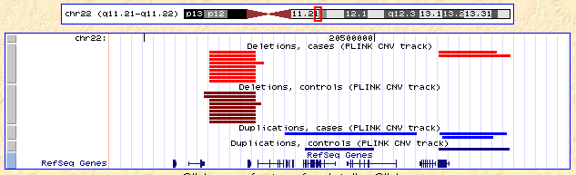Note that the CNVs are split by deletion versus duplication (red versus blue) and case versus control (light versus dark).

Additionally, a poor-man's version of this plot can be obtained with the command

     --cnv-seglist

which produces a file

     plink.cnv.seglist

which, for the CNV list above, can be seen here. Deletions and duplications are represented by + and - symbols at the start of each CNV; case and control status is represented as A and U.

Finally, it is also possible to report CNVs annotated by the regions or genes they span (see --cnv-verbose-report-regions described below.

Listing intersected genes and regions

With the --cnv-intersect (or --cnv-exclude) command, you can add the flag

     --cnv-report-regions

which will create a file

     plink.reg

listing only the regions that intersect (or do not intersect) with any of the CNVs (given the filtering and overlap commands that might also be specified). For example, to obtain a list of genes that are intersected by a rare case singleton deletions over 500kb (i.e. event seen only once)

 plink --cfile mydata 
       --filter-cases
       --cnv-freq-exclude-above 1
       --cnv-del
       --cnv-kb 500
       --cnv-report-regions
       --cnv-intersect glist-hg18

Alternatively, the command

     --cnv-verbose-report-regions

produces a verbose form of plink.reg, which does not just list the regions or genes intersected but lists the specific segmental CNVs also. This can be used in conjunction with, for example,

     --cnv-subset genes.txt

in order to produce reports on specific genes of interest. For example if genes.txt contained

     HES4
     ISG15

then

 plink --cfile mydata 
       --cnv-verbose-report-regions 
       --cnv-intersect glist-hg18 
       --cnv-border 20
       --cnv-subset genes.txt

would produce a file

     plink.reg

that, for each gene/region, contains the following fields

     FID        Family ID
     IID        Individual ID
     PHE        Phenotype
     CHR        Chromosome code
     BP1        Start position (base-pair)
     BP2        Stop position (base-pair)
     TYPE       DELetion or DUPlication
     KB         Kilobase length of CNV
     OLAP       Overlap (extent of CNV covered by gene)
     OLAP_U     Union overlap (ration of intersection to union)
     OLAP_R     Region overlap (extent of gene covered by CNV)

that might contain something like the following report


  RANGE (+/- 20kb )  [ 1 924206 925333 HES4 ]
       FID   IID   PHE  CHR        BP1      BP2  TYPE      KB     OLAP   OLAP_U   OLAP_R
      P001     1     2    1     789258  1232396   DUP   443.1  0.09281  0.09281        1
      P002     1     1    1     826576  1304312   DEL   477.7  0.08609  0.08609        1
      P003     1     2    1     864765  1913364   DUP    1049  0.03922  0.03922        1
      P004     1     1    1     890974  1258710   DUP   367.7   0.1118   0.1118        1

  RANGE (+/- 20kb )  [ 1 938709 939782 ISG15 ]
       FID   IID   PHE  CHR        BP1      BP2  TYPE      KB     OLAP   OLAP_U   OLAP_R
      P001     1     2    1     789258  1232396   DUP   443.1  0.09269  0.09269        1
      P002     1     1    1     826576  1304312   DEL   477.7  0.08598  0.08598        1
      P003     1     2    1     864765  1913364   DUP    1049  0.03917  0.03917        1
      P004     1     1    1     890974  1258710   DUP   367.7   0.1117   0.1117        1

That is, this is a list of any CNV that at least partially overlaps these two genes. The exact behavior can be modified with flags such as --cnv-del, --cnv-kb, --cnv-disrupt, --cnv-overlap, --filter-cases, etc.

Reporting sets of overlapping segmental CNVs

Finally, there are two option to group or report sets of segments that span a particular position. In the first case, use the option

     --segment-group

which takes all segments in a given region (whole genome unless otherwise specified) and forms "pools" of overlapping segments. Several pools of overlapping segments will be created; these will be listed in order of decreasing size (number of segments); note that the same segment can appear in multiple pools (e.g. if A overlaps with C, and B overlaps with C, but A and B do not overlap). The pools give information as described below.

The more restricted form of this command forms a single pool of all segments that overlap a particular position, which takes a single parameter of a marker name; typically these will be the dummy pos* markers created by the --cnv-make-map command.

     --segment-spanning pos119

In this case, for some made-up data, we see from the plink.cnv.summary file that there are 8 cases and 6 controls with a segment spanning a particular position, pos586

      CHR        SNP           BP      AFF    UNAFF
      ...        ...          ...      ...      ...
        1     pos586     16631570        8        6
      ...        ...          ...      ...      ...

In this case, there is unsurprisingly no association between segmental CNVs and disease: for example, the corresponding position in the plink.cnv.summary.mperm file shows an empirical p-value of 0.35, but of p=1 if adjusted for multiple testing (EMP2)

      CHR     SNP         STAT         EMP1         EMP2
      ...     ...          ...          ...          ...
        1  pos586     0.419408     0.351324            1
      ...     ...          ...          ...          ...

Naturally, one would usually be more interested in following up significantly associated regions of course... Nonetheless, if so desired we can see which segments (given any of the filtering specified) are spanning this position, with --segment-spanning, which gives the following:


    POOL       FID       IID    PHE  CHR        BP1       BP2       KB  TYPE  SCORE
      S1   PT-2378   PT-2378      2   12   16631570  16751087  119.517   DEL  10.23
      S1   PT-268D   PT-268D      2   12   16631494  16732162  100.668   DEL    9.3
      S1   PT-2M8O   PT-2M8O      1   12   16631441  16751082  119.641   DEL  31.23
      S1   PT-2FZ9   PT-2FZ9      2   12   16631436  16751045  119.609   DEL   15.2
      S1   PT-287D   PT-287D      1   12   16616579  17183201  566.622   DUP  200.3
      S1   PT-2C91   PT-2C91      2   12   16616579  16751045  134.466   DEL   14.3
      S1   PT-28A8   PT-28A8      1   12   16616579  16751045  134.466   DEL    8.3
      S1   PT-2FPB   PT-2FPB      1   12   16616579  16714372   97.793   DEL   11.1
      S1   PT-28IG   PT-28IG      2   12   16616579  16708856   92.277   DEL   10.3
      S1   PT-2E5N   PT-2E5N      2   12   16614664  16715703  101.039   DEL   9.87
      S1   PT-2FVL   PT-2FVL      1   12   16614664  16751045  136.381   DEL  10.67
      S1   PT-2DYE   PT-2DYE      2   12   16614664  16715489  100.825   DEL  11.82
      S1   PT-264I   PT-264I      2   12   16614664  16751045  136.381   DEL   14.2
      S1   PT-25WZ   PT-25WZ      1   12   16591338  16715767  124.429   DEL   14.7
      S1       CON        14    8:6   12   16631570  16708856   77.286    NA     NA
      S1     UNION        14    8:6   12   16591338  17183201  591.863    NA     NA

For CNV data (in contrast to shared segments based on homozygosity or IBD sharing) the extra fields of TYPE (deletion or duplication) and SCORE (some metric of quality/confidence of CNV call) are also presented.

Here we see the 14 segments listed, 8 cases and 6 controls. The CON and UNION lines at the end of the pool give the consensus region (i.e. shared by all segments) and the total distance spanned by all. The PHE field gives the phenotype for each individual.

Note that the way in which the dummy markers are selected will effectively mean that every possibly unique position, in terms of counts of segments, is evaluated. The actual base pair regions of any dummy marker is itself probably not of interest: given a sigificant (set of) SNPs, the strategy would be to select any one and generate the corresponding pool to see what and where the association maps to.

This document last modified Wednesday, 25-Jan-2017 11:39:26 EST

Whole genome association analysis toolset

Rare copy number variant (CNV) data