FIR filters

Linear-phase signal filters

Command	Description
`FILTER`	Apply a FIR filter to one or more signals
`FILTER-DESIGN`	Display filter properties

`FILTER`

Applies a linear-phase FIR filter to a signal

This command modifies the in-memory signal, by applying a finite impulse response (FIR) filter, which can be either a low-pass, high-pass, band-pass or band-stop filter.

Parameters

Core parameters are as follows:

Parameter	Example	Description
`sig`	`sig=C3,F3`	Restrict analysis to these channels
`bandpass`	`bandpass=0.3,35`	Band-pass filter between 0.3 and 35 Hz
`lowpass`	`lowpass=35`	Low-pass filter with cutoff of 35 Hz
`highpass`	`highpass=0.3`	High-pass filter between 0.3 and 35 Hz
`bandstop`	`bandstop=55,65`	Band-stop filter between 0.3 and 35 Hz
`fft`	Use FFT to implement the filter (this is now the default)

By default, the FILTER command uses the Kaiser window approach to define the filter, which requires the two following parameters:

Parameter	Example	Description
`ripple`	`ripple=0.01`	Ripple (as a proportion)
`tw`	`tw=1`	Transition width (in Hz)
`tw`	`tw=0.5,5`	Separate lower and upper transition widths for a bandpass filter (in Hz)

Note that if using bandpass tw=lwr,upr then you need to specify two values for ripple also (althogh these can be similar).

Ripple and stopband attenuation

The ripple parameter is related to stopband attenuation by the relation A = -20log10(ripple), such that a ripple=0.01 corresponds to -40 dB stopband attenuation.

Alternative filters

Alternatively, it is possible to

read the FIR coefficients in from a file
use the window method to design a FIR with a fixed filter order, using either a Bartlett, Hann, Blackman or rectangular window
use a narrow-band Gaussian filter, defined by a center frequecy and FWHM (full-width half-maximum) bandwidth, with ngaus
use an IIR Buttworth or Chebyshev filter

Parameter	Example	Description
`file`	`file=fir1.txt`	Read FIR coefficients from a file

`order`	`order=30`	Fix the FIR filter order
`rectangular`		Specify a rectangular window
`bartlett`		Specify a Bartlett window
`hann`		Specify a Hann window
`blackman`		Specify a Blackman window
`ngaus`	`ngaus=12,2`	Specify a narrow-band Gaussian filter (center frequency, FWHM)
`butterworth`	`butterworth=4`	A Butterworth IIR filter of fixed order (see below)
`chebyshev`	`chebyshev=4,1`	A Chebyshev IIR filter of fixed order and ripple factor (see below)

IIR filters

Butterworth and Chebyshev (type I) filters require one of bandpass=f1,f2, bandstop=f1,f2, lowpass=f1 and highpass=f1 options. Butterworth takes a single parameter, the filter order; Chebyshev takes two: order and the ripple factor epsilon - see the above link for a definition of how the ripple factor relates to passband ripple in dB. Chebyshev filters are sharper than the Butterworth filter, whereas Butterworth filters control passband ripple. Note that both IIR introduce phase delays: in general, FIR filters are probably preferable choices.

Output

After running FILTER, the in-memory signal for a filtered channel will represent the filtered signal. No explicit output is generated by the FILTER command.

Examples

As a first example, here we apply a bandpass filter to the EEG channel C3, with transition frequencies of 0.3 and 35 Hz, using a FIR filter designed via the Kaiser window method with a ripple parameter (ripple) of 0.01 and a transition width parameter (tw) of 0.5 Hz:

FILTER sig=C3 bandpass=0.3,35 ripple=0.01 tw=0.5

In this second example, we use lunaR to copy a signal, apply different bandpass filters to each duplicate (corresponding to delta, theta, alpha, sigma and beta frequency bands) and then plot the results. Here we use the individual nsrr02 from the tutorial dataset. In R, where we assume that the current directory is the one in which we unzipped the tutorial dataset (i.e. and so the s.lst sample-list is present), we'd enter the following:

library(luna)
lattach( lsl( "s.lst" ) , "nsrr02" )

nsrr02 : 14 signals, 10 annotations, 09:57:30 duration

For simplicity, we first drop all signals except EEG using SIGNALS:

leval( "SIGNALS keep=EEG" )

nsrr02 : 1 signals, 10 annotations, 09:57:30 duration

We then duplicate this signal using COPY five times, giving new labels to each:

leval( "COPY sig=EEG tag=DELTA" )
leval( "COPY sig=EEG tag=THETA" )
leval( "COPY sig=EEG tag=ALPHA" )
leval( "COPY sig=EEG tag=SIGMA" )
leval( "COPY sig=EEG tag=BETA" )

By the end, the message in the console reads:

nsrr02 : 6 signals, 10 annotations, 09:57:30 duration

Using lchs(), we confirm that all channels have been appropriately added:

lchs()

[1] "EEG"       "EEG_DELTA" "EEG_THETA" "EEG_ALPHA" "EEG_SIGMA" "EEG_BETA"

We then apply the FILTER command to apply a different band-pass filter to each of the channels:

leval( "FILTER sig=EEG_DELTA bandpass=0.5,4 tw=1 ripple=0.02" )
leval( "FILTER sig=EEG_THETA bandpass=4,8   tw=1 ripple=0.02" )
leval( "FILTER sig=EEG_ALPHA bandpass=8,12  tw=1 ripple=0.02" )
leval( "FILTER sig=EEG_SIGMA bandpass=12,15 tw=1 ripple=0.02" )
leval( "FILTER sig=EEG_BETA  bandpass=15,30 tw=1 ripple=0.02" )

We then epoch the data using lepoch():

ne <- lepoch()

nsrr02 : 6 signals, 10 annotations, 09:57:30 duration, 1195 unmasked 30-sec epochs, and 0 masked

We can use the ldata() function to pull out epochs of data for all 6 signals (i.e. as specified by giving lchs() as the second argument), e.g. here for epoch 135:

d <- ldata( 135 , lchs() )

Looking at the first few rows of the returned data frame d:

> head(d)
               INT   E      SEC        EEG EEG_DELTA   EEG_THETA  EEG_ALPHA
1 4020.00->4050.00 135 4020.000 -0.4901961 -3.473108 -0.06260304  3.4154174
2 4020.00->4050.00 135 4020.008 -2.4509804 -3.452390 -0.53536473  2.2660953
3 4020.00->4050.00 135 4020.016 -4.4117647 -3.307357 -1.13706143  0.4709635
4 4020.00->4050.00 135 4020.024 -5.3921569 -3.051824 -1.76561958 -1.5923434
5 4020.00->4050.00 135 4020.032 -6.3725490 -2.678883 -2.30284877 -3.4422047
6 4020.00->4050.00 135 4020.040 -7.3529412 -2.188535 -2.65204775 -4.5915269
   EEG_SIGMA   EEG_BETA
1 -1.9357408 -0.2801375
2 -2.7737269  1.0227155
3 -2.3793805  1.6093081
4 -0.9104402  0.8806983
5  0.9774931 -0.6320931
6  2.4513626 -1.3668775

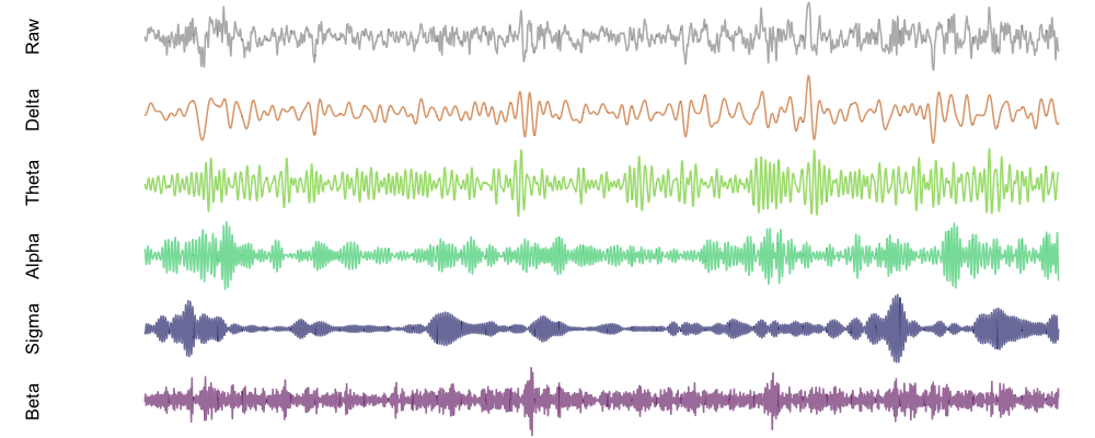
We can plot a data frame in this format with a R's internal functions, such as:

f1 <- function(d) {
par(mfcol=c(6,1),mar=c(0,5,0,0))
plot( d$EEG , type="l" , col=rgb(50,50,50,100,max=255) , axes=F , ylab="Raw" )
plot( d$EEG_DELTA , type="l" , col=rgb(200,100,00,150,max=255) , axes=F , ylab="Delta" )
plot( d$EEG_THETA , type="l" , col=rgb(100,200,0,150,max=255) , axes=F , ylab="Theta" )
plot( d$EEG_ALPHA , type="l" , col=rgb(0,200,100,150,max=255) , axes=F , ylab="Alpha" )
plot( d$EEG_SIGMA , type="l" , col=rgb(0,0,100,150,max=255) , axes=F , ylab="Sigma" )
plot( d$EEG_BETA ,  type="l" , col=rgb(100,0,100,150,max=255) , axes=F , ylab="Beta" )
}

Then, running f1( d ) will produce this plot (although, note that different signals are not uniformly scaled in this particular representation):

`FILTER-DESIGN`

Frequency and impulse responses for FIR filters designed via the Kaiser window method

Filters specified by the FILTER command use the Kaiser window method to design the filter. The FILTER-DESIGN command (or Luna --fir option) can be used to show the properties of these filters.

This command does not depend on any EDFs to be present, and so can be run without a sample-list or EDF (see the example below).

Parameters

Parameter	Example	Description
`fs`	`fs=256`	Sampling rate

`bandpass`	`bandpass=0.3,35`	Band-pass filter between 0.3 and 35 Hz
`lowpass`	`lowpass=35`	Low-pass filter with cutoff of 35 Hz
`highpass`	`highpass=0.3`	High-pass filter with cutoff of 0.3 Hz
`bandstop`	`bandstop=55,65`	Band-stop filter between 0.3 and 35 Hz

The FIR design design approaches are as for the FILTER command: either through the window method (with either a Kaiser window -- tw and ripple -- or fixing the FIR order) or reading from a file:

Parameter	Description
`ripple`	Ripple (as a proportion)
`tw`	Transition width (in Hz)

`file`	Read FIR coefficients from a file

`order`	Fix FIR order
`rectangular`	Specify a rectangular window
`bartlett`	Specify a Bartlett window
`hann`	Specify a Hann window
`blackman`	Specify a Blackman window

Output

Per-filter basics (strata: none)

Variable	Description
`FIR`	Label for FIR filter (constructed from input parameters)
`FS`	Sampling rate (from `fs` input parameter)
`NTAPS`	Filter order (number of taps)

Filter coefficients (strata: F x TAP)

Variable	Description
`TAP`	Tap
`W`	Filter coefficient

Frequency response characteristics (strata: F x FIR)

Variable	Description
`F`	Frequency (Hz)
`FIR`	FIR filter label
`MAG`	Magnitude
`MAG_DB`	Magnitude (dB)
`PHASE`	Phase

Impulse response (strata: FIR x SEC)

Variable	Description
`F`	Time (seconds)
`FIR`	FIR filter label
`IR`	Impulse response

Example

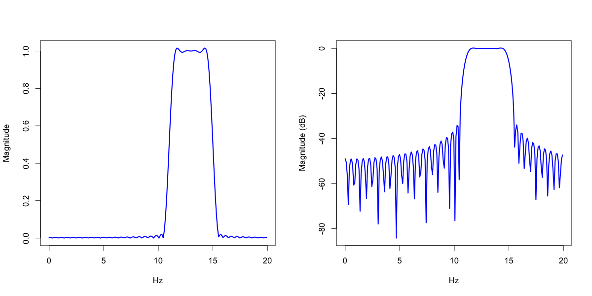
Consider a band-pass filter in the sigma band, 11 to 15Hz, applied to a signal with 200 Hz sampling rate. Transition frequencies 11Hz and 15Hz have -6dB attenuation (i.e. 50% amplitude ratio).

If specifying the --fir option, Luna expects the parameters above via standard input, e.g. piped from the echo shell command, with the output still sent to a database out.db:

echo "fs=200 bandpass=11,15 ripple=0.02 tw=1" | luna --fir -o out.db

Examining the out.db, we see that this command produces the following output:

destrat out.db

--------------------------------------------------------------------------------
out.db: 1 command(s), 1 individual(s), 7 variable(s), 4207 values
--------------------------------------------------------------------------------
  command #1:   c1  Mon Feb 25 16:11:40 2019    FIR-DESIGN  
--------------------------------------------------------------------------------
distinct strata group(s):
  commands      : factors           : levels        : variables 
----------------:-------------------:---------------:---------------------------
  [FIR-DESIGN]  : FIR               : 1 level(s)    : FS NTAPS
                :                   :               : 
  [FIR-DESIGN]  : F FIR             : 1025 level(s) : MAG MAG_DB PHASE
                :                   :               : 
  [FIR-DESIGN]  : FIR TAP           : 365 level(s)  : W
                :                   :               : 
  [FIR-DESIGN]  : FIR SEC           : 765 level(s)  : IR
                :                   :               : 
----------------:-------------------:---------------:---------------------------

The first stratum (FIR) gives the sampling rate (FS) as input, and the derived order of the filter (NTAPS):

destrat out.db +FIR-DESIGN -r FIR

ID    FIR                        FS      NTAPS
.     BANDPASS_11..15_0.02_1     200     365

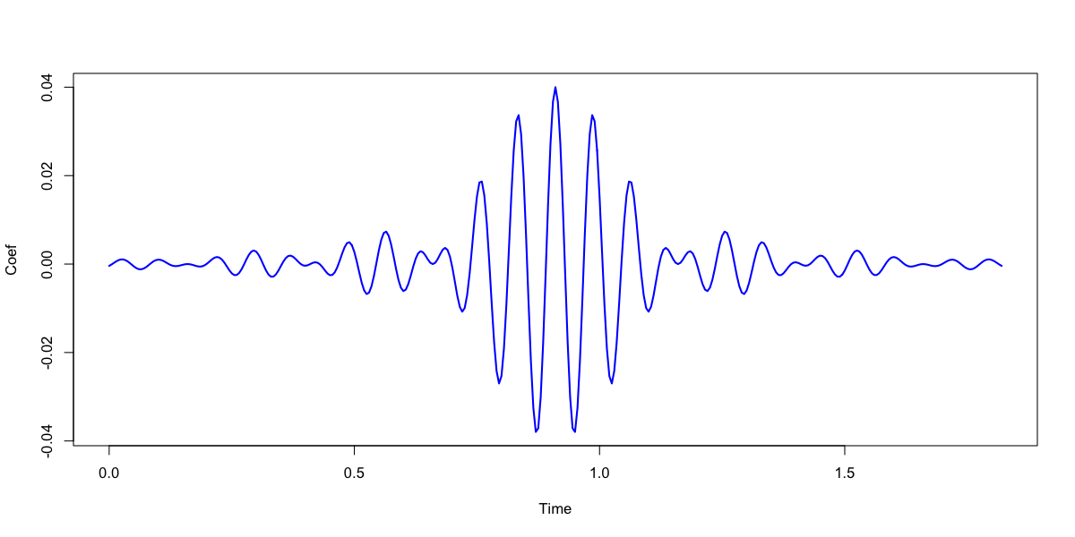
The actual filter coefficients are in the stratum defined by FIR x TAP:

destrat out.db +FIR-DESIGN -r FIR TAP > fir.txt

In R, we can plot the filter coefficients:

w <- read.table("fir.txt",header=T)
plot( w$TAP/200 , w$W , type="l", lwd=2, col="blue", ylab="Coef", xlab="Time" )

The amplitude (magnitude) response of the filter is in the F x FIR stratum:

destrat out.db +FIR-DESIGN -r F FIR > fir2.txt

In R:

d <- read.table("fir2.txt", header=T)
d <- d[ d$F < 20 , ]
par(mfcol=c(1,2))
plot(d$F, d$MAG   , type="l",lwd=2,col="blue", xlab="Hz",ylab="Magnitude")
plot(d$F, d$MAG_DB, type="l",lwd=2,col="blue", xlab="Hz",ylab="Magnitude (dB)")