Prediction models

Feature-based prediction models

The PREDICT command is designed to take a pre-existing linear model with predictors (features) corresponding to metrics that Luna emits (e.g. spectral power, etc). In conjunction with a suitable script to estimate those metrics, PREDICT combines model and data to make a prediction. Essentially, this framework aims to provide a one-step procedure for going from (raw) PSG/EEG data as input, to a model-based prediction as output.

For example, one PREDICT model supports the prediction of the so-called brain age index using the NREM EEG, based on a model from Sun et al (2019). This model has also been incorporated into the Moonlight viewer. Over time, different models as well as support for model classes beyond linear models will be compiled here.

Command	Description
Overview	Overview of the PREDICT framework
`PREDICT`	Make a prediction given a model and pre-calculated features
Models	Currently supported models

Overview

The PREDICT command assumes the following components:

a model specification that defines a set of features, along with their weights and population means/standard deviations, used to construct a feature vector for each individual/EDF
a paired Luna script that generates the required features, using the CACHE record mechanism to pass those feature values to the PREDICT command
optionally, a dataset of normalized values from the training dataset, to support kNN-based imputation of missing data

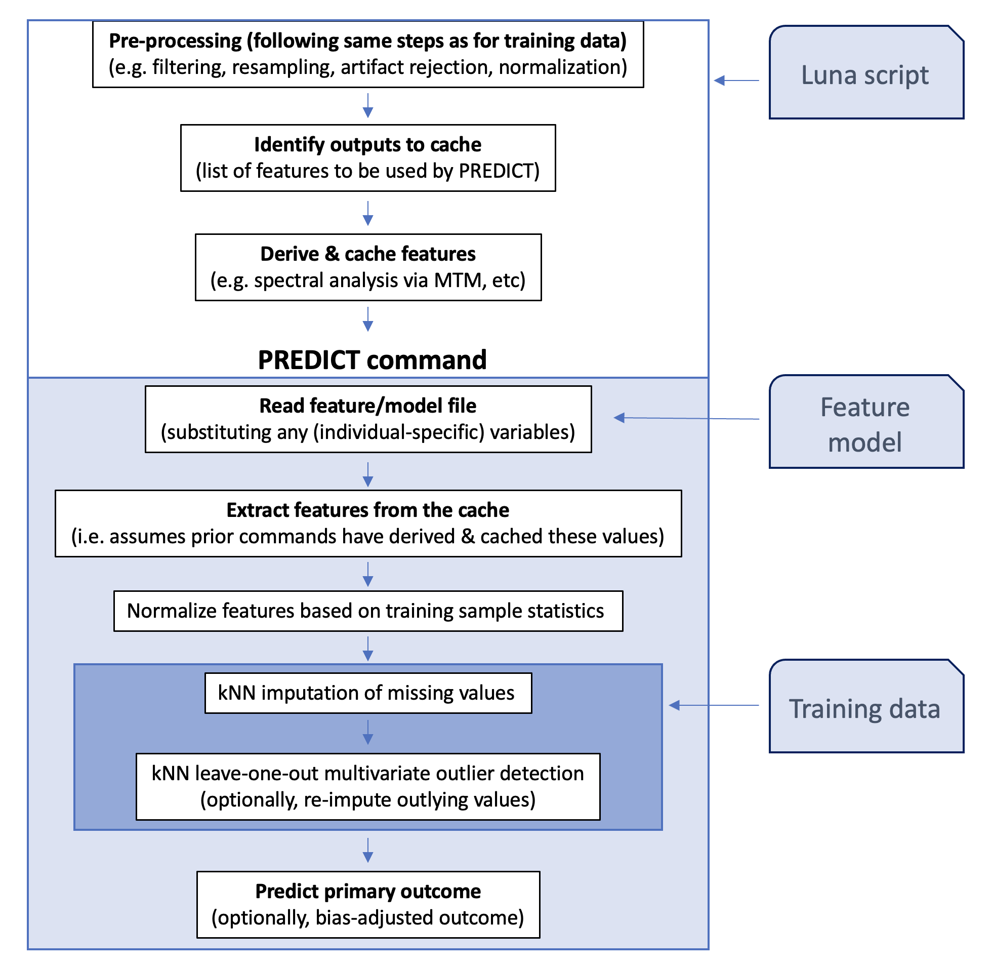
The primary workflow is as follows:

Info

As a downstream user of the PREDICT command (i.e. when using pre-defined models to make predictions) most of the details on this page are unnecessary and you can skip ahead to the documentation on the main PREDICT command itself. The details below are for reference, aimed at individuals who want to use this framework to bring their own models into this framework.

Model specification file

A model specification file contains the following components:

feature definitions
definitions for special variables (e.g. model intercept), e.g.

Each feature definition has the following terms:

Term	Example	Description
label	`delta_theta_mean_C_N3`	Arbitrary label for the feature
`CMD`	`CMD=MTM`	Specifies the Luna command used to generate the feature
`VAR`	`VAR=RATIO`	Specifies the exact Luna variable from that command
`STRATA`	`STRATA=STG/N3,B1/DELTA,B2/THETA`	Specifies any additional strata
`CH`	`CH=${cen}`	Specifies which channel(s) to consider
`m`	`m=0.52`	Population mean for this feature
`sd`	`sd=0.23`	Population standard deviation for this feature
`b`	`b=-0.7`	Coefficient for this feature (for a standardized metric)
`LOG`	`LOG=1`	Use the natural log of this feature, `Z = sign(X) * log1p(\|X\|)`
`REQ`	`REQ=1`	Set to 1/0 to indicate if a feature is required to be non-missing
`CHS`	`CHS=C3+F3,C4+F4`	Specifies pairwise channels, e.g. for metrics such as coherence (here two pairs: C3-F3 and C4-F4)
`DIR`	`DIR=1`	Set to 1/0 to indicate if a pairwise statistic is directional, i.e. if m(A,B) = -m(B,A) versus m(A,B) = m(B,A)
`VALUE`	`VALUE=${x}`	Set a feature based on a variable rather than a cache value

Typically, only the first eight terms will be used. The terms CHS and DIR are only applicable for channel-pairwise metrics, e.g. coherence. As a concrete example, this is one line (of 13 terms in the whole model) from the Sun et al. model:

delta_theta_mean_C_N3
 CMD=MTM  VAR=RATIO  STRATA=STG/N3,B1/DELTA,B2/THETA  CH=${cen}
 b=1.3862 m=1.2243 sd=0.4581

That is, this feature is a ratio between two band powers (delta and theta) from N3 sleep, averaged across all central channels listed in the variable ${cen} (note, this variable does not need to be labelled ${cen}, it could be any valid Luna variable name, e.g. ${s}). The label name (delta_theta_mean_C_N3) is aribitrary, used only to identify the feature, i.e. it could equally be ftr01 etc. (It should not contain spaces or an equals sign, however.) Here, the feature is described across multiple lines, although it is also permissable to use a single line. The label must come first; all other attributes, that will be in the form of key=value pairs, can be in any order.

Using the cache

The cache is a mechanism whereby one Luna command can pass information to another Luna command during the processing of a single recording - i.e. a temporary store specific to an individual.

When used with PREDICT, there are three primary points at which the cache is invoked:

via the CACHE record statement, to tell Luna which metrics to track
when a tracked command is run, any tracked values will be cached
when PREDICT runs, based on the model specification file details, values will be pulled from the cache and used to build the vector of predictors for that individual

To take the specific case above, the first component might be:

CACHE cache=c1 record=MTM,RATIO,B1,B2,CH,STG

The record argument expects values in the form/order: command, variable, one or more strata. This names a cache c1 (i.e. the same cache will be passed to PREDICT) and instructs Luna to cache any RATIO values emitted by the MTM command that have the associated strata of B1, B2, CH and (in this particular case) STG. Here, RATIO is the ratio of two band powers (B1 / B2 ), which will be defined for a given channel CH. By default, any RATIO variable will always have at least these three associated strata, B1, B2 and CH: e.g. B1=DELTA, B2=ALPHA and CH=C3_M2. Here, we additionally specify a stratifying factor of STG, corresponding to sleep stage. This is a user-defined strata specified via the TAG command, used to track N2 versus N3 metrics calculated in the same script. The tag makes N2 and N3 metrics distinct, otherwise new calls to MTM would overwrite the output associated with previous ones in the same run.

Given the above CACHE command, Luna will cache those values from any outputs that match all these conditions (i.e. for that command, variables and strata combination):

MASK ifnot=N3
RE preserve-cache
TAG STG/N3
MTM sig=C3,C4 ratio1 ratio=DELTA/THETA,DELTA/ALPHA

After running the MTM command above, Luna will cache the four following strata, each defined for four factor/level pairs, for the RATIO variable (that is, a single number representing the power ratio for that channel and pair of bands for N3 sleep):

CH/C3 B1/DELTA B2/THETA STG/N3
CH/C4 B1/DELTA B2/THETA STG/N3
CH/C3 B1/DELTA B2/ALPHA STG/N3
CH/C4 B1/DELTA B2/ALPHA STG/N3

The final step involving the cache is when PREDICT retrieves cached values for that recording, given a set of feature definitions, e.g.:

delta_theta_mean_C_N3
 CMD=MTM  VAR=RATIO  STRATA=STG/N3,B1/DELTA,B2/THETA  CH=${cen}
 b=1.3862 m=1.2243  sd=0.4581

Luna will pull the first two of the four values cached above, as both match the level values for the factors B1, B2 and STG. The channel specification (CH) is handled separately from the other strata (which are specified by the STRATA keyword). Assuming the ${cen} was previously defined to be cen=C3,C4, this will retrieve estimates of N3 delta/theta power ratio from both channels and then take the average. The CH keyword can handle one or multiple channels, but will always emit a single (averaged) value.

Restructing/freezing with caches

In the above example, note that the RE command had the special option preserve-cache. By default, RE and THAW would otherwise wipe the cache. When using a cache, this is typically not what one wants, i.e. if we wish to retain the cached values until a subsequent PREDICT command.

Consider the following example (given here not as a full working example, but just a skeletal script): if we wished to use sigma band power from both N2 and N3 (from the Welch PSD command, which emits a variable also called PSD with strata defined by band B and channel CH alongside a further STG stratum that aligns with the TAG commands below):

CACHE cache=c1 record=PSD,PSD,B,CH,STG

% pre-process whole signal
FILTER sig=CZ bandpass=0.3,35 tw=1 ripple=0.01

FREEZE F1

% get N2 metrics
TAG STG/N2
MASK ifnot=N2
RE preserve-cache
PSD sig=CZ

THAW tag=F1 preserve-cache

% get N3 metrics
TAG STG/N3
MASK ifnot=N2
RE preserve-cache
PSD sig=CZ

% clear STG, else PREDICT output would have a STG/N3 stratum
TAG STG/.

% predict given both N2 and N3 metrics 
PREDICT cache=c1 model=model1.txt

In the above, the cached metrics from N2 would be lost if we thawed the previous F1 freeze (i.e. as that freeze did not contain the cached values). That is, the preserve-cache option decouples the cache from the typical snapshot mechanism for returning to a former state. A similar logic applies with the restructure command. The simple rule is: if building a script that uses PREDICT and a cache, add preserve-cache to THAW and RE.

Using variables

In the above example, channel CH is set to a Luna variable (here ${cen}), which allows more flexibility, i.e. one does not need to edit the model specification file if running on a dataset with a different label.

In addition, to include features in a predictive model that are not derived from Luna commands per se (and will therefore not be in the cache), you can use the VALUE keyword when defining a model: e.g. to include a covariate for male versus female sex:

male_sex
 VALUE=${male} b=-0.22 m=0.48 sd=0.5

This assumes that a variable called ${male} will have been defined for that individual (even if it is defined as missing for that individual). Such a variable is specified in the same way as any other Luna variables, e.g. on the command line

luna file1.edf male=1 -o out.db < predict.txt

or (more likely, in the context of multiple individuals) in a vars files

luna s.lst vars=covar.txt -o out.db < predict.txt

where covar.txt is a tab-delimited file, with ID as the first column, and a column labelled male (note: case-sensitive) as one of the other columns:

ID     age   male   site
id001  12    1      A
id002  16    0      A
id003   9    .      B
id004   6    1      B
...

If you specify a VALUE term for a particular feature, you should not also specify CMD, VAR or STRATA terms as well, as those relate to searching the cache.

Special variables

As well as defining the core terms, the model specification file also specifies a few special variables, in the format

variable <- value

e.g.

intercept <- 42

The primary special variables are

Variable	Description
`observed`	If known, the observed value (e.g. chronological age) to be used in output, and bias-adjustment
`intercept`	The model intercept
`data`	The filename of the feature matrix data file (for kNN imputation) - can also be given as `data` as a option to `PREDICT`
`knn`	The number of nearest neighbours to consider when running kNN imputation
`minf`	The minimum number of non-missing features required to run the model
`softplus`	Apply the `softplus` function to the output (0/1=N/Y)
`log1p`	Apply `log1p()` scaling to all inputs (0/1=N/Y)

There are also some special labels expected that can be used to describe the model (currently not directly used by Luna, but adding to the model file can help to document the model for users):

Variable	Description
`title`	A title for the model
`reference`	A PMID or similar reference for the model/data
`outcome`	The type/unit of the predicted outcome, e.g. Age (years)
`type`	Type of model (linear/logistic) - currently only linear models supported
`training`	Brief note about the training data or procedure

Bias-adjustment models

Some models (including Sun et al. mentioned above) require a bias-adjustment term (e.g. as described here).

Variable	Description
`bias_correction_slope`	Coefficient for bias adjustment model (b)
`bias_correction_intercept`	Intercept (c)
`bias_correction_term`	Observed/known value (e.g. chronological age), same as `${observed}` (a)

If these terms are found in a model specification file, then a bias-adjusted version of the prediction (Y1) will be output as well as the raw estimate (Y).

This particular form of bias adjustment uses the observed value of the output variable, as is appropriate in the context of biological/brain age prediction models, i.e. where chronological age will be known, and it is the difference between predicted and chronological age that is the outcome of primary interest.

Given b, c and a as defined above, and an initial prediction y, the bias-adjusted value y1 is simply defined as

 Y1 = Y - ( B * A + C )

If PREDICT is given the above terms in the model file (along with the observed value A), it will automaticall calculate and output Y1 as well as Y.

Reference data

If a reference dataset is included with the data option (to support kNN imputation) it must have the following format:

each row is one individual/observation, each column is one feature; all features are whitespace-delimited
first row starts with # followed by number of rows (observations) and columns (features), e.g.
```
# 2936   13
```
second row also starts # and then lists all feature labels (that must match the terms in the model file exactly)
subsequent rows contain the numeric values, expected to be standardized (i.e. each column has mean of 0, SD of 1)

See this file for an example.

PREDICT

Make a prediction based on a specified model and cached Luna metrics

See the overview above for a high-level description of this command, and how it fits into a broader paradigm of using Luna to support model-based prediction. PREDICT is typically not used alone, but rather needs to be paired with a) a model specification and b) a Luna script with upstream commands to compute and cache the features (predictors) used in the model.

Internally, the steps are:

PREDICT reads the model specification file and swaps in any variables (similarly to how Luna parses command scripts); this is done separately for each individual, i.e. meaning that model files can contain variables that vary between different individuals
it then attempts to find values for the specified model features; typically these will be from the cache, but if a variable exists with (exactly) the same name (i.e from a vars file) then it will be used; otherwise, the default is for PREDICT to search the cache
next, it checks there are enough non-missing features, as specified by REQ or minf in the model file
it then standardizes all features based on population mean/SD values (which are always included in a model file)
PREDICT uses a simple k-nearest neighbour (kNN) approach to impute missing values, based on knn=10 neighbours by default; kNN imputation is only performed if a reference data file has been attached
if a reference dataset is available, PREDICT also uses it to identify outlier features, by dropping each non-missing feature in turn, re-imputing it, and then calculating the difference (observed - imputed) in SD units. If the distance exceeds the th threshold set, the observed values are taken to be outliers, and replaced with their imputed values
using standardized features, PREDICT then makes a prediction based on the implied linear model; if the model file specifies it, a subsequent bias-adjustment procedure is applied (see above)

Cacheless mode

If features have been pre-computed and are all available in a simple text file, PREDICT can run quickly in cacheless mode, i.e. directly taking feature values as variables rather than running Luna commands on the raw data. In this way, you could use PREDICT as a standalone command (on the assumption that features.txt has columns defined to match each defined term in model.txt):

luna s.lst vars=features.txt -o out.db -s PREDICT model=model.txt

See below for an example of this approach.

Parameters

Primary parameters

Option	Example	Description
`model`	`models/m1.txt`	Model/feature specification filename
`cache`	`p1`	Specify a prior cache name
`data`	`models/m1.data`	Data set (to support kNN imputation)
`th`	4	Absolute Z-value distance to trigger re-imputation

Secondary parameters

Option	Example	Description
`drop`	`ftr2,ftr3`	Drop one or more features from the model
`dump-model`		Dump the model to standard output

Outputs

Individual-level output (strata: none):

Variable	Description
`NF`	Number of features
`NF_OBS`	Number of features observed (non-missing)
`OKAY`	Flag for whether sufficient non-missing features were observed (0/1=N/Y)
`Y`	Default prediction
`Y1`	Optional, bias-adjusted prediction
`YOBS`	Observed value for outcome, if known

Feature-level output (strata: FTR)

Variable	Description
`X`	Raw value of this feature
`Z`	Normalized feature value
`D`	kNN-derived distance for any non-missing feature
`IMP`	Flag for whether this feature was imputed, i.e. if missing (0/1=N/Y)
`REIMP`	Flag for whether this feature was "re-imputed"(*), i.e. if an outlier (0/1=N/Y)
`B`	Feature coefficient (from the model, fixed for all individuals)
`M`	Feature mean (from the model, fixed for all individuals)
`SD`	Feature standard deviation (from the model, fixed for all individuals)

(*) Calling this 're-imputed' doesn't really make much sense, but the output is stuck with this nomenclature for now.

Example

As a full working example, we will consider the model described in Sun et al (2019). This model contains 13 features based on the NREM sleep EEG. It was trained on 2,532 individuals to predict an individual's age.

The model specification file is available here.
The Luna script used to extract the features and run the PREDICT command is available here.
The above repository also contains the datafile for kNN imputation here.

For simplicity, imagine these files are called m-features.txt, m-luna.txt and m-data.txt respectively, available (relative to the current working folder) in the folder models/.

The Luna script a) sets up the cache, b) does some pre-processing, c) extracts metrics for N1, then N2, then N3 sleep, using the freeze/thaw mechanism to swap between stages, and then d) runs PREDICT to make a predicton.

If p1.lst is a sample list pointing to the EDF and staging annotations for one 69 year-old individual, then we could run:

luna p1.lst age=69 cen=C3,C4 th=3 mpath=models/ -o out.db < m-luna.txt

The Luna script expects the variables ${th} and ${mpath} to be defined, as these are passed as parameters to the PREDICT command, as well as ${cen}, to indicate which (central mastoid-referenced EEG) channels to derive metrics from. The model specification file further expects the variables ${age} and ${cen} to be defined. In practice, ${age} (which obviously varies between individuals) would be specified via a vars file.

Re-referencing on-the-fly

Note that in this particular case, the channels were not contra-lateral mastoid referenced, whereas the above m-luna.txt assumes they are (inspect the script to see). Rather than edit the script, or use two versions, one can splice in additional commands to Luna, by using standard command-line tools: i.e. what we actually ran was (the other arguments replaced with ... here):

echo "REFERENCE sig=C3 ref=A2 & REFERENCE sig=C4 ref=A1" | cat - m-luna.txt | luna p1.lst ...

This is equivalent to

luna p1.lst ... < m-luna.txt

but if we had editted the first lines of m-luna.txt to include the extra REFERENCE commands. The above is equivalent to:

cat m-luna.txt | luna p1.lst ...

and so here we use cat - m-luna.txt to concatenate the standard input (here from a prior echo) with the Luna script, and then all of that gets piped into Luna, i.e. in the form:

echo "extra first commands go here" | cat - script.txt | luna p1.lst ...

This script contains multiple commands and generates a lot of console output. It is always worth reviewing in test cases that the script it performing as expected. The final PREDICT command gives the following messages to the console:

 CMD #37: PREDICT
   options: cache=p1 data=models/m-data.txt model=models/m-features.txt sig=* th=3
  read 13 terms and 8 special variables from models/m-features.txt
  creating 2936 x 13 reference feature matrix from models/m-data.txt
  applying softplus scaling to predicted values

  predicted value (Y) = 59.8799
  bias-corrected predicted value (Y1) = 70.613
  observed value (YOBS) = 69

That is, this individual had an observed age of 69 years, and a (bias-adjusted) estimated age (based on the NREM EEG) of 70.6 years.

The primary outputs are available in out.db:

destrat out.db +PREDICT

ID     NF    NF_OBS   OKAY    Y       Y1      YOBS
id01   13    13       1       59.879  70.613  69

where NF is the number of feautres used in the model. Depending on the model used, either Y or Y1 should be considered as the primary output.

We can view the individual features:

destrat out.db +PREDICT -r FTR

ID   FTR                                B      M     SD      X       D      Z IMP REIMP
id01 COUPL_OVERLAP_C               -0.804  366.3  191.7  270.0  -0.178 -0.502   0     0
id01 DENS_C                        -1.665  4.513  1.911  3.486  -0.857 -0.537   0     0
id01 alpha_bandpower_kurtosis_C_N2 -3.184  7.331  2.598  6.263  -0.108 -0.411   0     0
id01 alpha_bandpower_mean_C_N1      2.291  0.068  0.047  0.046  -1.395 -0.465   0     0
id01 delta_alpha_mean_C_N3         -1.348  1.344  0.548  0.808  -0.266 -0.975   0     0
id01 delta_bandpower_kurtosis_C_N2 -1.868  17.01  4.071  10.47  -0.496 -1.607   0     0
id01 delta_bandpower_mean_C_N3     -2.620  1.445  0.618  0.857  -0.279 -0.949   0     0
id01 delta_theta_mean_C_N3          1.386  1.224  0.458  0.744  -0.310 -1.049   0     0
id01 kurtosis_N2_C                 -0.052  2.851  1.349  1.362  -0.047 -1.103   0     0
id01 kurtosis_N3_C                 -1.247  1.086  0.576  0.335  -0.368 -1.302   0     0
id01 sigma_bandpower_kurtosis_C_N2  1.247  15.19  4.749  18.11   0.741  0.615   0     0
id01 theta_bandpower_kurtosis_C_N2 -3.744  7.461  2.557  6.222   0.440 -0.484   0     0
id01 theta_bandpower_kurtosis_C_N3  0.157  5.364  2.045  2.301  -0.962 -1.496   0     0

The order of columns has been changed (default is alphabetical) for easier viewing above:

the first three give the coefficient, mean and population SD and will be identical for all individuals (i.e. these are directly from the model file)
X is the observed value of the feature (in this case, all derived from cached Luna commands)
D is the distance in SD units for the expected value of the feature based on kNN imputation based on all non-missing features but excluding this one
Z is the normalized (potentially imputed) final version used in the prediction equation (i.e. multipled by B)
IMP and REIMP indicate whether the final Z value was imputed, either because it was missing (IMP) or an outlier based on D (REIMP)

If particular features appear to be consistently noisy or biased, they can be dropped from the model by adding the option drop=F1,F2 where F1 and F2 are two features, for example.

Building feature matrices to re-run models

If a script takes a long time to compute features, or if you have a large sample, and you wish to re-run models (e.g. changing parameter settings) it can be advantageous to extract all features from the output to make a single text input file.

We first pull the values X (i.e. the raw features used by the model, but after averaging across channels) as follows:

destrat out.db +PREDICT -c FTR  -v X > ftr.txt

One adjustment needs to be made so that the column headers then line up exactly with the feature labels:

ID      X.FTR_COUPL_OVERLAP_C   X.FTR_DENS_C          ...
id01    270                     3.48598130841121      ...

The above file has 13 columns (plus an ID field) but the labels (following default destrat output practices have the variable/factor name X.FTR_ at the front of each column label. We can strip these, either manually, as using something as follows:

sed 's/X\.FTR_//g' < ftr.txt > ftr2.txt

ID      COUPL_OVERLAP_C   DENS_C          ...
id01    270               3.48598130841121      ...

In practice, you'd want to be very careful that the IDs or other values don't values that match X.FTR_ etc, but this works for now. We can then re-run the single PREDICT step as follows:

luna p1.lst vars=ftr2.txt age=69 cen=C3,C4 -o out2.db -s PREDICT model=models/m-features.txt data=models/m-data.txt th=3

which will run effectively instantaneously, yielding the same output as above:

  bias-corrected predicted value (Y1) = 70.613
  observed value (YOBS) = 69

Note that in practice, age (and potentially other information such as the central channel labels to use) could instead be kept in a file (with multiple individuals on different rows), e.g. covar.txt

ID      age     male    cen
id01    69      1       C3,C4
id02    73      0       CZ
id03    56      1       C3,C4
...

luna p1.lst vars=ftr2.txt,covar.txt -o out2.db -s PREDICT model=models/m-features.txt data=models/m-data.txt th=3

which, again, will give the same output.

Now we can easily change parameters, e.g. varying th or dropping particular terms. For example, here we might drop both spindle-related metrics: running the same command as above but adding to PREDICT

drop=DENS_C,COUPL_OVERLAP_C

This has a slight impact on the predicted value:

  bias-corrected predicted value (Y1) = 68.6742
  observed value (YOBS) = 69

We can see the values have been imputed:

destrat out2.db +PREDICT -r FTR -v IMP X Z

ID    FTR                           IMP   X           Z
id01  COUPL_OVERLAP_C                 1   NA     -0.015
id01  DENS_C                          1   NA      0.391
id01  alpha_bandpower_kurtosis_C_N2   0   6.263  -0.411
id01  alpha_bandpower_mean_C_N1       0   0.046  -0.465
id01  delta_alpha_mean_C_N3           0   0.809  -0.976
id01  delta_bandpower_kurtosis_C_N2   0   10.47  -1.607
id01  delta_bandpower_mean_C_N3       0   0.858  -0.950
id01  delta_theta_mean_C_N3           0   0.744  -1.049
id01  kurtosis_N2_C                   0   1.363  -1.103
id01  kurtosis_N3_C                   0   0.335  -1.302
id01  sigma_bandpower_kurtosis_C_N2   0   18.11   0.615
id01  theta_bandpower_kurtosis_C_N2   0   6.222  -0.485
id01  theta_bandpower_kurtosis_C_N3   0   2.302  -1.497

The NA for X in the top two rows indicated they were dropped from the original model as observed variables, i.e. set to missing then imputed. As expected these values deviate from the observed values somewhat : -0.015 and 0.391 instead of -0.502 and -0.537 and have resulted in a slightly lower estimated age. In a larger sample, one could use the above framework to perform sensitivity analyses, etc, e.g. to see if some terms increase or decrease noise in predictions significantly.

Viewing the original channel-level features

Finally, just to connect the features (internally cached metrics passed to PREDICT) with the "standard" Luna outputs, we can look at the rest of the out.db file, which will contain the same values that were cached. The one difference is that PREDICT internally averaged over multiple channels, and so we'll need to do that here to check that things line up.

To take a few examples: first spindle density, which has the label DENS_C in the model:

destrat out.db +PREDICT -r FTR/DENS_C -v X

ID    FTR      X
id01  DENS_C   3.48598

From the main SPINDLES output, we know it was stratified by F and CH (as always for spindle density) but also STG (because this was added in the script via TAG STG/N2 before the spindles command):

destrat out.db +SPINDLES -r F CH STG -v DENS

ID     CH     F  STG     DENS
id01   C3  13.5   N2  3.65421
id01   C4  13.5   N2  3.31776

As expected, the mean of these two values equals the value of X from PREDICT, i.e. (3.65421 + 3.31776)/2 = 3.48598.

To consider a second example: the delta/alpha N3 power ratio: delta_alpha_mean_C_N3. From the model file, we can see the definition:

delta_alpha_mean_C_N3
  CMD=MTM  VAR=RATIO  STRATA=STG/N3,B1/DELTA,B2/ALPHA  CH=${cen}

i.e. from the RATIO variable of the MTM command, and based on a stratum defined by the two power bands, a stage and channels:

destrat out.db +MTM -r B1/DELTA B2/ALPHA STG/N3 CH -v RATIO

ID       B1     B2  CH   STG     RATIO
id01  DELTA  ALPHA  C3    N3   0.78152
id01  DELTA  ALPHA  C4    N3   0.83614

We are therefore expecting X to be the mean of these, namely (0.78152+0.83614)/2 = 0.80883. From PREDICT itself, the averaged value was:

destrat out.db +PREDICT -r FTR/delta_alpha_mean_C_N3 -v X

ID                      FTR            X
id01  delta_alpha_mean_C_N3    0.8088296

which matches expectations.

Models

Currently, in its initial release, only a single model is supported - more will be added soon.

Label	Model	Link
SUN2019	"Brain-age" prediction for adults	repo

SUN2019

Sun et al (2019) uses 13 NREM sleep EEG features to provide a robust estimate of "brain age". The difference between predicted and observed age is labelled the brain age index. The model was trained on over 2,500 adults aged 18 to 80.