SOAP

Self-contained modelling and evaluation of sleep staging

Command	Description
SOAP	Single-observation accuracies and probabilities
REBASE	Use SOAP to translate between epoch lengths (e.g. 20 to 30 second manual staging)
PLACE	Use SOAP to localize "lost" stage annotations

This suite of commands are based around the SOAP (Single Observation Accuracies and Probabilities) function in Luna. In brief, SOAP generates a battery of epochwise features based on one or more channels, and then fits a simple model (e.g. linear discriminant analysis) to those data, with the observed stages (i.e. passed as annotations) as the outcomes. If the signal is a) of sufficient quality, and b) is related to observed sleep stages via the computed features, then SOAP should be able to generate a model that explains the observed stages relatively well. This can be assessed, for example, via the kappa coefficient between observed and predicted stages. Inability to derive a good-fitting model is therefore indicative of problems with the stages and/or signals.

Info

The SOAP command requires existing stage annotation, i.e. similar to the HYPNO command (whether these existing annotations are from manual scoring, or from an external, automated staging algorithm). That is, it does not predict sleep stages from scratch. For automated staging, see Luna's POPS command.

Overall, the SOAP model can be viewed in two ways: 1) as a tool to check the consistency between signals & staging - implemented in the SOAP command, or 2) as a tool to manipulate/use the existing staging, on the assumption that stages and signals are largely consistent, i.e. as in PLACE and REBASE. In addition, the SOAP command can be used to fill-in modest amounts missing staging, e.g. if a sufficient number of representative epochs have been manually scored.

SOAP

Single observation stage accuracies and probabilities

Fits the SOAP model to predict stage labels, based on a simple LDA (or QDA) model for a set of epoch-level features, typically based on spectral analysis. Outputs of this model can indicate if there is gross inconsistency between stage labels and signal data (assuming a signal that would be expected to track strongly with sleep stage, i.e. typically an EEG).

The standard typical usage is very simple, as it uses a default feature/model set, i.e. something like:

luna s.lst -o out.db -s SOAP sig=C3_M2 

However, we first introduce the fuller set of features and models.

Features

Each feature (or feature set) is calculated per epoch for the channel(s) specified after each keyword:

Parameter	Arguments	Description
SPEC	lwr=0.5 upr=25	Spectral decomposition via Welch's method
RSPEC	lwr=0.5 upr=25 z-lwr=0.5 z-upr=25	Relative spectral decomposition, normalized by range z-lwr to z-upr
VSPEC	lwr=0.5 upr=25	Variance of segment-to-segment power in each epoch
SLOPE		Spectral slope
SKEW		Signal skewness
KURTOSIS		Signal kurtosis
HJORTH		Second and third Hjorth parameters
FD		Fractal dimension
PE		Permutation entropy statistics (with embedding dimension 3 - 7)
MEAN		Simple channel mean, e.g. for pulse signal

That is,

 SPEC C3 lwr=0.5 upr=25

will implicitly specify 99 features (log-scaled power values from 0.5 to 25 Hz at default value of 0.25 Hz intervals for C3). It is possible to specify the features from multiple channels, e.g.

 SPEC C3 C4 lwr=0.5 upr=25

which will add 2 x 99 features to the epoch-by-feature matrix.

These additional keywords do not require any channels to be listed, but instead operate on the currently set of features:

Parameter	Arguments	Description
TIME	order=2	Add time-tracks (up to order N)
DENOISE	lambda=0.5	Total-variation denoiser, replace features; lambda in SD units, as per TV
DENOISE2	lambda=0.5	Total-variation denoiser, duplicate features; lambda in SD units, as per TV
NC	10	Required: number of components to extract from all features

Of the above, the NC is the most important - this determines the final variables entered into the LDA/QDA model, i.e. the top N principal components from the epoch-by-feature matrix.

Models

A SOAP model is defined by one or more feature sets , which implies a certain number of variables (columns) in the final epoch-by-feature matrix. As noted, the NC option then takes the entire epoch-by-feature matrix (which can reflect a mix of features from one or more channels), normalizes it (potentially after removing outliers), fits a PCA and then extracts the top e.g. 10 components to be used in a LDA model predicting stage labels given these components.

You can create a text file to specify which SOAP features to use, and use the model=file.txt argument for SOAP to use it. Alternatively, you can use a default model. If nothing else is specified (or model=_1) this is the model used:

SPEC <sig> lwr=0.5 upr=25 
NC 10

where <sig> is replaced by the value of sig after the SOAP command. This perform spectral analysis per epoch and then summarizes the values as 10 principal components per epoch.

A second vanilla model can be used by specifying model=_2 :

SPEC <sig> lwr=0.5 upr=25
RSPEC <sig> lwr=5 upr=20 z-lwr=30 z-upr=45
SLOPE <sig> 
SKEW <sig>
KURTOSIS <sig>
FD <sig>
PE <sig>
DENOISE2 lambda=0.5
TIME order=4
NC 10

This adds a suite of additional features, but still extracts only 10 components from the final set.

For most circumstances, where the goal is to use SOAP to spot chronically poor stage/signal alignment, the default model appears to work well enough (i.e. with typically high kappa values for sufficiently high-quality datasets).

Parameters

Primary options:

Parameter	Example	Description
sig	C3_M2	Signal to use for the SOAP model
epoch		Write epoch-level outputs (i.e. posterior probabilities, stage predictions)

Secondary/advanced options:

Parameter	Example	Description
model	m1.txt	Read explicit model/feature file, if not using the default; or _1 or _2 for internal models, _1 is default
lights-off	23:00:10	Specify a lights_off time, i.e. ignore before
lights-on	08:00:00	Specify a lights_on time, i.e. ignore after
th	3	Remove epochs with component outliers at this SD level
trim	10	Trim leading/trailing wake, to keep N epochs before/after first/final sleep
end-wake	120	Threshold for trimming excessive WASO (mins) - see HYPNO notes
end-sleep	5	Threshold for trimming excessive WASO (mins) - see HYPNO notes
pc	0.05	Require components to have p-value below this, from one-way ANOVA with stage
qda		Use QDA instead of LDA
dump-svd	f	Write PCA/SVD components to f.U, f.W and f.V
dump-features	f.txt	Write epoch by feature matrix to f.txt
force-reload		Add if re-running SOAP when using lunaR R library

Output

Individual-level summary metrics (strata: none)

Variable	Description
K	5-class kappa
K3	3-class kappa (NREM / REM / Wake )
ACC	5-class accuracy
ACC3	3-class accuracy
MCC	5-class Matthew's correlation coefficient
MCC3	3-class MCC
F1	5-class F-1 score
F13	3-class F-1
PREC	5-class precision
PREC3	3-class precision
RECALL	5-class recall
RECALL3	3-class recall
PREC_WGT	Weighted precision
RECALL_WGT	Weighted recall

Epoch-level output (option: epoch; strata: E)

Variable	Description
DISC	0/1 for observed/predicted discordance (5-class)
DISC3	0/1 for observed/predicted discordance (3-class)
INC	0/1 for inclusion in final model
PP_N1	N1 posterior probability
PP_N2	N2 posterior probability
PP_N3	N3 posterior probability
PP_NR	NREM posterior probability
PP_R	REM posterior probability
PP_W	Wake posterior probability
PRED	Predicted stage
PRIOR	Original observed stage

Stage-level output (strata: SS)

Variable	Description
DUR_OBS	Observed stage duration
DUR_PRD	Predicted stage duration
F1	Stage-specific F-1 score
PREC	Stage-specific precision
RECALL	Stage-specific recall

Component-level output (strata: VAR)

Variable	Description
INC	0/1 for whether component included
PV	Stage-component oneway ANOVA p-value

Stage-transition metrics (strata: SS x ETYPE)

Variable	Description
ACC	Accuracy
N	Number of observed instances

Above, the SS factor is is sleep stage (N1, N2, etc) as well as ALL. The ETYPE factor is as follows: the epoch under consideration is the second of the three (here labelled A):

Epoch-type label	Description
OAO	All epochs, i.e. O means anything
AAA	Epochs flanked by similar epochs, i.e. also A
AAX	Epochs just prior to a stage transition, i.e. X implies not A
XAA	Epochs just after a stage transiton
XAX	Singleton epochs, i.e. with different stages before and after
TRN	Epochs at any type of transition (AAX, XAA or XAX)

Epoch-level confusion matrix (strata: NSS x PRED x OBS )

Variable	Description
N	Number of epochs
P	Proportion of epochs, conditional on observed stage

Here NSS is either 3 or 5 for 3-class or 5-class assignments. OBS and PRED are the observed and predicted stage labels respectively. The information in this table is the same as reported in the console.

Example

See this vignette to see SOAP in action.

Running SOAP on an NSRR tutorial individual:

luna s.lst 2 -o out.db -s SOAP sig=EEG

This fits the default model (10 PSC components from the per-epoch PSD power spectra):

 CMD #1: SOAP
   options: sig=EEG
  using LDA for primary predictions
  read 1 feature specifications (99 total features on 1 channels) from _1
  resampling channel EEG from sample rate 125 to 128
  set epochs to default 30 seconds, 1195 epochs
  set 0 leading/trailing sleep epochs to '?' (given end-wake=120 and end-sleep=5)
  applying Welch with 4s segments (2s overlap), using median over segments
  expecting 99 features (for 1195 epochs) and 1 channels
  standardizing X
  final feature matrix X: 99 features over 1195 epochs
  of 1195 total epochs, valid staging for 1195, and of those 1195 passed outlier removal
  outlier counts: flat, Hjorth, components, trimmed -> total : 0, 0, 0, 0 -> 0
  re-standardizing X after removing bad epochs
  epoch counts: N1:11 N2:399 N3:185 R:120 W:480
  final epoch counts: N1:11 N2:399 N3:185 R:120 W:480
  final count of valid epochs is 1195
  retaining 9 of 10 PSCs, based on ANOVA p<0.01
  LDA: removed 0 missing values, 1195 remaining, with 9 features

Luna then reports the 5-class confusion matrix:

  Confusion matrix: 5-level classification: kappa = 0.81, acc = 0.87, MCC = 0.81

       Obs:     N1     N2     N3      R      W    Tot
  Pred:  N1      7      4      0      0      8   0.02
         N2      2    315     13     28      7   0.31
         N3      0     42    170      0      1   0.18
          R      2     30      1     89      7   0.11
          W      0      8      1      3    457   0.39
       Tot:   0.01   0.33   0.15   0.10   0.40   1.00

Followed by the 3-class one:

 Confusion matrix: 3-level classification: kappa = 0.86, acc = 0.92, MCC = 0.86

         Obs:   NR      R      W    Tot
  Pred:   NR   553     28     16    0.50
           R    33     89      7    0.11
           W     9      3    457    0.39
        Tot:  0.50   0.10   0.40    1.00

Even with this simple model, the kappa coefficients are high here, meaning that stages and signals align well. See the above-referenced vignette for examples of when this is not the case.

We can plot the posterior probabilities, e.g. using lunaR:

k <- ldb( "out.db" )
d <- k$SOAP$E

# a small fix needed for now...
d$FLAG <- 0  

# function to make the plot
lpp2( d )

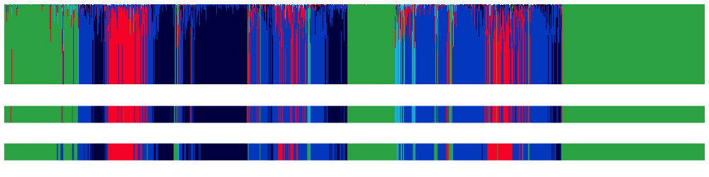
The top panel shows the posterior probabilities; the middle is the most likely stage from SOAP; then lower is the observed stage. [W, R, NREM = green, red, blue(s)].

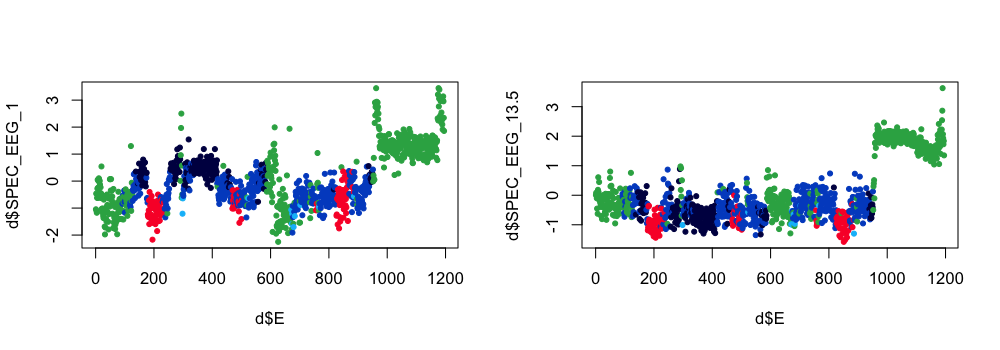
We can also extract the raw feature matrix, and the components:

luna s.lst -o out.db -s SOAP sig=EEG epoch dump-features=f.1 dump-svd=cmp

In R:

ss <- ldb( "out.db" )$SOAP$E

Loading raw feature and plotting using observed stage label to color the points:

d <- read.table( "f.1" , header=T ) 
png( file="soap-dump1.png" , width=1000, height=350 , res=100 , units="px" )
par(mfcol=c(1,2))
plot( d$E , d$SPEC_EEG_1 , pch=20 , col= lstgcols( ss$PRIOR ) )
plot( d$E , d$SPEC_EEG_13.5 , pch=20 , col= lstgcols( ss$PRIOR ) ) 
dev.off()

Plotting components: here are the first two components:

d <- read.table( "cmp.U" , header=T )
par(mfcol=c(1,2))
plot( d$E , d$C1 , pch=20 , col= lstgcols( ss$PRIOR ) )
plot( d$E , d$C2 , pch=20 , col= lstgcols( ss$PRIOR ) )

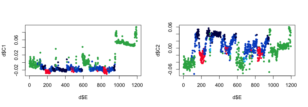
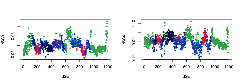
Here are the third and fourth components:

par(mfcol=c(1,2))
plot( d$E , d$C3 , pch=20 , col= lstgcols( ss$PRIOR ) )
plot( d$E , d$C4 , pch=20 , col= lstgcols( ss$PRIOR ) )

REBASE

Translate existing (manual) staging between different epoch durations (e.g. from 20 second to 30 seconds epoch) using the SOAP model

Parameters

Parameter	Example	Description
dur	10	Required epoch duration for the emitted stages

All other parameters are as for SOAP, described above.

Output

All outputs are as for SOAP, described above, except the epoch duration will vary.

Example

See this vignette for an example.

PLACE

Temporally align existing staging signal data

Parameters

Option	Value	Description
stages	stage.txt	.eannot stype file with stage data
edf-overlap	0.1	Require that at least 10% of the EDF is spanned
stg-overlap	0.5	Require that at least 50% of the staging data is spanned
out	Output the best-aligned stages to an .eannot of this name
force		Force alignment, even if equal number of epochs in stage file and EDF

Additionally, the standard SOAP options can be used to modify the type of SOAP analysis used by PLACE.

Output

Individual-level output (strata: _none)

Variable	Description
K	Best kappa
OFFSET	Estimated offset
OLAP_EDF	Proportion of EDF spanned by best alignment
OLAP_STG	Proportion of staging data spanned by best alignment
OLAP_N	Number of overlapping epochs in best alignment

Per-putative offset output (stratum: OFFSET)

Variable	Description
FIT	0/1 for whether model fit for this offset, i.e. enough valid stages, etc
K	SOAP Kappa
K3	SOAP 3-class kappa
NE	Number of epochs in alignment
NS	Number of unique stages for this alignment
OLAP_EDF	Proportion of EDF spanned
OLAP_STG	Proportion of staging data spanned
OLAP_N	Nember of epochs spanned
S	Kappa relative to best kappa (i.e. max = 1)
S3	3-class kappa relative to best (i.e. max = 1)
SS	Stage count string, e.g. ?:782,N1:1,N2:108,N3:11,R:45,W:248

Example

See this vignette for an example.

luna s.lst 2 -s STAGE min > s.1

Here we will remove the first 200 epochs from the staging data:

awk ' NR > 200 ' s.1 > s.2

luna s.lst 2 -o out.db -s PLACE stages=s.1 force

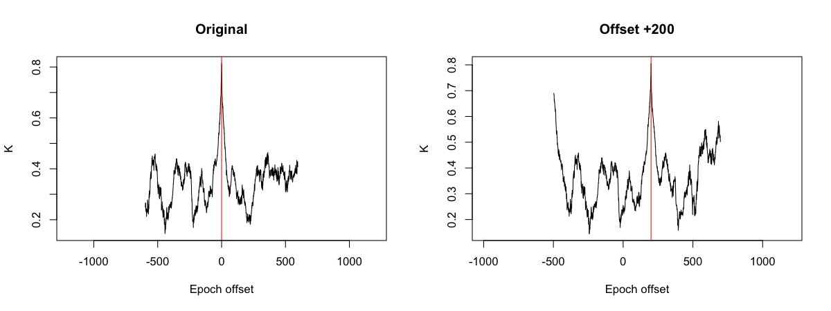
  optimal epoch offset = +0 epochs (kappa = 0.813969)
  which spans 1195 epochs (of 1195 in the EDF, and of 1195 in the input stages)

In the second case, the observed stage data is now shorter, and placement is ambiguous (we no longer need to force analysis here either):

luna s.lst 2 -o out.db -s PLACE stages=s.2 sig=EEG 

  optimal epoch offset = +200 epochs (kappa = 0.805433)
  which spans 995 epochs (of 1195 in the EDF, and of 995 in the input stages)

We see that PLACE correctly identified the offset, as +200 epochs.

destrat out.db +PLACE -r OFFSET > o.1
destrat out2.db +PLACE -r OFFSET > o.2

In R:

d1 <- read.table("o.1",header=T,stringsAsFactors=F)
d2 <- read.table("o.2",header=T,stringsAsFactors=F)
par(mfcol=c(1,2))
plot( d1$OFFSET , d1$K , type="l" , xlab="Epoch offset" , ylab = "K" , main="Original" ) 
abline( v = 0 , col = "red" ) 
plot( d2$OFFSET , d2$K , type="l" , xlab="Epoch offset" , ylab = "K" , main="Offset +200") 
abline( v = 200 , col = "red" )