EEG microstates

Implementation of the modified K-means approach to EEG microstate analysis

Command	Description
`MS`	EEG microstate analysis
`--kmer`	(Group-level) permutation-based analysis of state sequences
`--cmp-maps`	Group/individual map spatial analysis
`--label-maps`	Label maps given a template
`--correl-maps`	Spatial correlations between maps

`MS`

Fits the modified k-means clustering to EEG data

This implementation follows the seminal publication by Pascual-Marqui et al. (1995) as well as a guide and code by Poulsen et al.

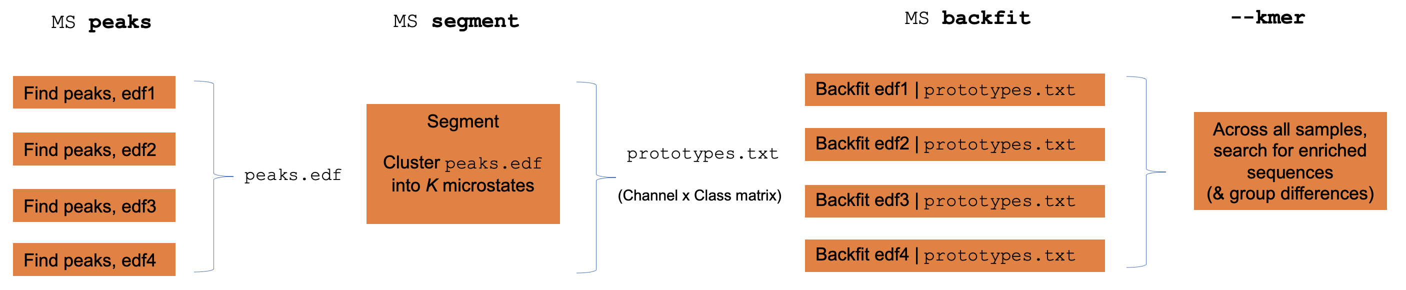
Briefly, the MS workflow follows these steps:

extracts global field power (GFP) peaks from EEG signals (that must previously have been average-referenced)
cluster GFP maps (segmentation) to a small number of prototypes, e.g. K = 2,3,4, etc, using a polarity-invariant (modified k-means clustering, in which prototypes are based on the first eigenvector of the class-specific covariance)
backfit the prototype maps to all original sample points
perform temporal smoothing (relabelling short segments)
calculate various statistics per individual
finally, per individual or at the group level, search for enriched sequences of states as well as group differences (kmer analysis)

Individual versus group level analyses

Luna operates one EDF at a time, although often one wants to apply EEG microstate clustering across multiple individuals. To achieve this, Luna splits out the core functions of the MS command (GFP peak extraction, segmentation, backfitting and kmer/sequence enrichment) into sub-commands that can be run individually to faciliate group-level analysis.

Warning

There are numerous methodological subtleties to EEG microstate analysis, and this Luna implementation does not purport to support all of these differences.

Parameters

Single-subject clustering

Option	Example	Description
`gfp-max`	`3`	Exclude GFP peaks with amplitude 3 SD units above the mean
`gfp-min`	`1`	Exclude GFP peaks with amplitude 1 SD units below the mean
`gfp-kurt`	`1`	Exclude GFP peaks with spatial kurtosis 1 SD above the mean
`npeaks`	`5000`	Number of GFP peaks to extract
`all-points`		Use all EEG points for clustering, rather than selecting only GFP peaks (can be a lot of data...)
`dump-gfp`	`gfp.txt`	Report all GFP peaks to this file
`standardize`		Standardize GFP maps within individual
`verbose`		Report verbose output
`epoch`		Perform backfitting epoch-by-epoch

Multi-subject clustering

GFP peak detection:

Option	Example	Description
`peaks`	`p1.edf`	Write GFP peaks to this EDF
`npeaks`	1000	Number of peaks to extract per individual
`pmin`	-250	EDF physical minimum for new peaks EDF
`pmax`	250	EDF physical maximum for new peaks EDF

Segmentation parameters:

Option	Example	Description
`segment`	`sol.txt`	Perform microstate clustering (segmentation) and write best-fitting prototype maps to this file
`k`	`2,3,4,5,6`	Fit models for these values of K (number of states)

Backfitting parameters:

Option	Example	Description
`backfit`	`sol.4`	Backfit prototype maps to EEG data and calculate various statistics
`backfit`	`sol.4,B,C,A,D`	Backfit prototype maps, specifying label order explicitly (for columns in `sol.4`)
`min-msec`	`20`	Iteratively replace short states (default 20 msecs)

Output parameters:

Option	Description
`write-states`	File to write state sequences to
`add-sig`	Add a new 0/1 channel to the EDF for each microstate
`add-annot`	Add an internal annotation for each microstate

Sequence analysis parameters:

Option	Example	Description
`kmers`	`3,6,1000`	Ssequence enrichment analysis (per individual) 3 args = 1) min, 2) max kmer length, 3) number of permututations

Outputs

Individual-level outputs for the best-fit solution (strats: none)

Variable	Description
`GEV`	Global variance explained
`OPT_K`	Optimal K (based on GEV)
`LZW`	Lev-Zimpel-Welch complexity of state sequences
`SE1`	Sample entropy statistics `SE1,`SE2`, etc

Per-cluster statistics (for the best-fit model) (strata: K)

Variable	Description
`COV`	Coverage (proportion of points spanned)
`DUR`	Mean state duration (msec)
`OCC`	Cccurrences per second
`SPC`	Spatial correlation
`GEV`	Global explained variance
`GFP`	Global field power
`N`	Number of sample-points spanned , i.e. unstandardized `COV`

Per-solution statistics, i.e. for a given value of K (strata: NK)

Variable	Description
`MSE`
`R2`
`SIG2`
`SIG2_MCV`

Prototype map (for best-fit soluition) (strata: CH x K)

Variable	Description
`A`	Element of A matrix

Prototype map (from each K solution) (strata: KN x CH x K)

Variable	Description
`A`	Element of A matrix

State transition probabilities for best-fit solution (strata: PRE x POST)

Variable	Description
`P`	Transition probability

Sequence enrichment (within individual) ( strata: L x S )

Variable	Description
`OBS`	Observed number of observations
`EXP`	Expected number of observations
`P`	Empirical enrichment significance value
`Z`	Empirical enrichment Z score
`SG`	Equivalence group label
`NG`	Number of sequences in the sequence's equivalence group (`SG`)
`W_OBS`	Within-equivalence group observed rate
`W_EXP`	Within-equivalence group expected rate
`W_P`	Within-equivalence group rate enrichment signifiance
`W_Z`	Within-equivalence group rate enrichment Z score

Sequence enrichment (within individual) equivalence groups ( strata: L x SG )

Variable	Description
`NG`	Number of members of this equivalence group
`OBS`	Observed number of observations
`EXP`	Expected number of observations
`P`	Empirical enrichment p-value
`Z`	Empirical enrichment Z score

Example

For a single individual/EDF, apply microstate analysis.

luna file.edf –o out.db –s MS sig=${eeg} k=2,3,4,5

Note, prior to to above command, we require that the EEG signals have already been average-referenced.

CMD #1: MS
 options: k=2,3,4 kmers=2,4,100 sig=*
 find GPF peaks
 calculating GFP for sample
 extracted 15997 peaks from 90000 samples (18%)
 segmenting peaks to microstates
 K=2 replicate 1/10... GEV = 0.658197 (new 2-class best)
 K=2 replicate 2/10... GEV = 0.658197 (new 2-class best)
 K=2 replicate 3/10... GEV = 0.658197
 K=2 replicate 4/10... GEV = 0.658197
 K=2 replicate 5/10... GEV = 0.658196
...
 based on GEV, now setting K=2 as the optimal segmentation
 K=3 replicate 1/10... GEV = 0.707564 (new 3-class best)
 K=3 replicate 2/10... GEV = 0.707566 (new 3-class best)
 K=3 replicate 3/10... GEV = 0.707569 (new 3-class best)
 K=3 replicate 4/10... GEV = 0.707566
 K=3 replicate 5/10... GEV = 0.707566
..
 K=4 replicate 10/10... GEV = 0.725835
 based on GEV, now setting K=4 as the optimal segmentation

 back-fitting solution to all time points
 smoothing: rejecting segments <= 20 msec

 kmers: considering length 2 to 4
 kmers: for 156 sequences, 41 equivalence groups
 kmers: running 100 replicates...

destrat out.db +MS -r CH -c K

ID     CH  A.K.A  A.K.B  A.K.C A.K.D
ID0001 Fp1 0.419  0.281  0.275 0.163
ID0001 Fp2 0.169  0.181  0.073 0.186
ID0001 AF3 0.395  0.266  0.215 0.187
ID0001 AF4 0.087  0.090 -0.073 0.231
ID0001 F7  0.266  0.212  0.228 0.065
ID0001 F5  0.309  0.268  0.243 0.111
ID0001 F3  0.291  0.237  0.183 0.131
ID0001 F1  0.065  0.046 -0.038 0.167
ID0001 F2 -0.002 -0.019 -0.142 0.210
ID0001 F4  0.005  0.041 -0.096 0.172
ID0001 F6  0.103  0.273  0.106 0.122

destrat out.db +MS -r K -v DUR COV

ID     K COV   DUR
ID0001 A 0.222 118.531
ID0001 B 0.202 106.553
ID0001 C 0.285 119.100
ID0001 D 0.291 119.325

Multi-subject clusterig

The first step is to extract all GFP peaks, by creating an aggregated EDF which contains only a fixed number of peaks per individual:

First we ensure there is no file named peaks.edf to start with:

rm -rf peaks.edf

Adding the peaks option to the MS command will then cause Luna to iterate over every individual in the s.lst sample list, and append the peaks for that individual to the end of the peaks.edf (updating the EDF header each time more records are added). Because we need to write the EDF header on encountering the first individual, we also need to manually specify the physical min/max values we expect to see across all subjects (pmin and pmax). Finally, we select the number of GFP peaks to extract with npeaks (here 5000), and an optional threshold whereby very large GFP peaks are ignored (gfp-th):

luna  s.lst -s MS peaks=peaks.edf gfp-th=1 npeaks=5000 pmin=-200 pmax=200

The aggregated EDF peaks.edf is therefore a temporary that contains data (peaks) from multiple individuals (in this case, 130 individuals from s.lst). Because it is only used in the MS analysis, we set the sample rate (arbitrarily) to 1 Hz. As a sanity check, as we extracted 5000 peaks for each of 130 individuals, we expect a total of 650,000 observations for the subequent EEG microstate clustering. Indeed, this is what we observe (i.e. assuming a

luna peaks.edf -s DESC

  duration: 180.33.20 | 650000 secs

Inspecting the GFP peaks across individuals

When combining data across individuals, it is important to ensure that peak amplitudes are broadly comparable across individuals. You can use the standard Luna summary tools such as SIGSTATS (i.e. to get RMS and Hjorth parameters) to achieve this (so long as the metric does not depend on the sampling rate that is). Because peaks.edf arbitrarily sets the "sample rate" to 1 Hz, and in this example we extracted 5000 peaks per individual, we can use a trick of setting the "epoch length" to 5000 seconds, and request an epoch-level analysis. This means that each "epoch" in the output in fact corresponds to all GFP peaks for one individual: e.g. from

luna peaks.edf -o out.db -s EPOCH dur=5000 & SIGSTATS epoch

You can inspect the channel-by-individual (CH by E) that results from this, to search for outlier individuals, etc, in which case it may be necessary to standardize GFP peaks prior to merging.

Next, we perform the primary MS segmentation of these collated GFP peaks. In this case we fix K to 4 and write the solution to the file sol.4:

luna peaks.edf -o out.db -s MS segment=sol.4 k=4

That is, the input to this step is peaks.edf rather than all the EDFs in s.lst, as the 130 individuals are already contained in it.

At this point, one might examine sol.4 visually, to determine which prototype corresponds to which canonical state (i.e. A, B, C, D, etc from the literature).

Next, we backfit this solution to the original data (i.e. s.lst) and extract various statistics:

luna s.lst -o out.db -s MS backfit=sol.4  write-states=states/s4-^

In the above command, we also specify write-states option, in order to save the sequence of microstates for each individual in a file (where ^ is replaced with the individual ID)

Labelling microstates

By default, the states are labelled A, B, C, D, etc, in the order they appear in the file sol.4, which will be arbitrary. Based on visual inspection, if the states have clear labels they can be explicitly labelled by adding the state labels after the file name (i.e. here, we know that sol.4 contains 4 states), if we see they correspond to B, A, C and D respectively:

backfit=sol.4,B,A,C,D

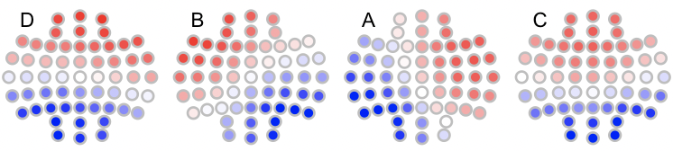
We can visualize the prototype maps, e.g. using ltopo.rb()

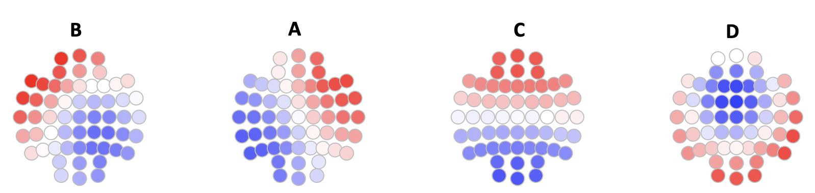
Here we see that the four states correspond to the canonical 4 states as often reported (for a K=4 solution in the EEG microstate literature).

--kmer

Apply state sequence permutation analysis across multiple individiuals and assess group differences

As well as applied within individual, the kmer option can be run "stand-alone", on the output from write-states from the MS command, if they are concatenated into a single file. The permutation occurs within individual, but the statistics (i.e. enrochment of specific k-mers) are aggregated across all people. In addition, if a binary phenotype is specified (via phe), then these statistics are calculated separately for CASES (phenotype == 1) and CONTROLS (phenotype == 0); furthermore, the difference between case and control statistics is evaluated for each metric and the empirical significance of all these terms is calculated.

Parameters

Option	Example	Description
`file`	`file=all.states`	Concatenated output from `write-states` (one row per individual)
`vars`	`vars=data.txt`	Tab-delimited file containing `ID` column and phenotypes
`phe`	`phe=DIS`	Pointer to a column of `data.txt` that is a 0/1 variable
`k`	`k=3`	Single k-mer length
`k1`	`k1=2`	Consider k-mers from `k1` to `k2
`k2`	`k2=4`	Consider k-mers from `k1` to `k2
`nreps`	`nreps=100`	Number of replicates

Output

Sequence enrichment (group-level) ( strata: L x S )

Variable	Description
`OBS`	Observed number of observations
`EXP`	Expected number of observations
`P`	Empirical enrichment significance value
`Z`	Empirical enrichment Z score
`SG`	Equivalence group label
`NG`	Number of sequences in the sequence's equivalence group (`SG`)
`W_OBS`	Within-equivalence group observed rate
`W_EXP`	Within-equivalence group expected rate
`W_P`	Within-equivalence group rate enrichment signifiance
`W_Z`	Within-equivalence group rate enrichment Z score

Sequence enrichment (group-level) equivalence groups ( strata: L x SG )

Variable	Description
`NG`	Number of members of this equivalence group
`OBS`	Observed number of observations
`EXP`	Expected number of observations
`P`	Empirical enrichment p-value
`Z`	Empirical enrichment Z score

Sequence enrichment (by phenotype) ( strata: PHE x L x S )

Variable	Description
`OBS`	Observed number of observations
`EXP`	Expected number of observations
`P`	Empirical enrichment significance value
`Z`	Empirical enrichment Z score
`SG`	Equivalence group label
`NG`	Number of sequences in the sequence's equivalence group (`SG`)
`W_OBS`	Within-equivalence group observed rate
`W_EXP`	Within-equivalence group expected rate
`W_P`	Within-equivalence group rate enrichment signifiance
`W_Z`	Within-equivalence group rate enrichment Z score

Sequence enrichment (by phenotype) equivalence groups ( strata: PHE x L x SG )

Variable	Description
`NG`	Number of members of this equivalence group
`OBS`	Observed number of observations
`EXP`	Expected number of observations
`P`	Empirical enrichment p-value
`Z`	Empirical enrichment Z score

Example

Continuing from the example above, we can test for enrichment of sequences by concatenating all state sequences across individuals: we had previously saved the sequences to text files (one line per individual) in the folder states/ and so can concatenate as follows:

cat states/s4* > all.states

Assuming that the file cc.txt contains a 0/1 encoded group indicator PHE in the first row and the individual ID labelled ID in the header, we can run various enrichment statistics and test for group differences (across all individuals) with the --kmer command:

echo "file=all.states vars=cc.txt phe=PHE k=4 nreps=100" | luna --kmer -o out.db

Hint

Note, here k is 4, but this is a different quantity from the K = 4 in the clustering segmentation. In this context, k of 4 means we consider sequences up to 4 states in length, e.g. ABAB, ABDA, ABCD, etc. (which could have fewer or more unique state labels at each position).

--cmp-maps

Group/individual map spatial analysis

Note that this function does not require or accept an EDF or sample list.

This command takes a set of microstate maps, along with an optional group/phenotype file (two groups only) and evaluates the topographical simiarity / dissimilarity of maps between groups/people, based on the summed spatial correlation between maps.

The starting point for this command is always running individual-level segmentation with the MS command.

First, we perform individual-level segmentation:

luna s.lst -o maps.db \
     -s  ' REFERENCE sig=${eeg} ref=${eeg}
           MS sig=${eeg} k=4 gfp-max=3 gfp-min=1 gfp-kurt=1  npeaks=5000 '

We then extract all maps/solutions from all individuals to a single text file: (swapping IDs to match phe.txt)

destrat maps.db +MS -r CH K > all.maps

For group-level tests, we require a tab-delimited file (e.g. phe.txt) with ID and some other column with a 0/1 field: (here DIS):

luna --cmp-maps -o out.db \
     --options file=all.maps vars=phe.txt phe=DIS nreps=1000

The output to the console may look like:

  of 125 total individuals, for DIS 68 cases, 57 controls and 0 unknown
  creating individual-by-individual global similarity matrix

  within-case similarity                       : 0.819118 p = 0.628372
  within-control similarity                    : 0.824668 p = 0.34965
  | within-case - within-control | similarity  : 0.00555053 p = 0.802198
  concordant / discordant pair similarity      : 0.984001 p = 0.478521

All four above statistics are evaluated empirically. There is likely some redundancy here: the primary ones are #3 and #4. (Arguably, #1 and #2 just help interpret a significant result from #3.).

From top to bottom, these statistics reflect the following questions::

are cases more similar to each other than we’d expect by chance (1-sided)
are controls more similar to each other than we’d expect by chance (1-sided)
are cases as similar to each other as controls are similar to each other? (2-sided, absolute difference)
are phenotypically concordant pairs more similar than discordant pairs? (1-sided, ratio)

To get individual level outputs (the mean similarity of that person vs all others):

destrat out.db +CMP-MAPS

ID          S
ID_0003     0.872831506350531
ID_0004     0.821114969439348
ID_0005     0.859732202249929
ID_0006     0.88057487661809
ID_0007     0.845507629897367
ID_0009     0.863454475897446
ID_0011     0.841742414155102
ID_0012     0.861049164391393
ID_0013     0.874618198441904
... etc ...

To run in template mode (i.e. comparing all individuals to a fixed template, rather than making a comparison between groups:

luna --cmp-maps -o out.db \
     --options file=all.maps vars=phe.txt phe=DIS nreps=1000 template=prime6

Here prime6 is a text file with the template map, as Luna outputs from segmentation: i.e. w/ a header row and tab-delimited columns:

CH    B          A        F         E          C          D
Fp1   0.181639   0.12153  0.29197   0.078162   0.183723   0.0652307
Fp2   0.053939   0.20571  0.25708  -0.100524   0.165446   0.0531564
AF3   0.206103   0.12500  0.20173   0.071661   0.20764   -0.0747048
AF4   0.055686   0.22630  0.1419   -0.143023   0.183976  -0.0930419
F7    0.206141  -0.00312  0.23955   0.201432   0.113696   0.101976
... etc ...

 running CMP-MAPS
  found 6 classes: B A F E C D
  read 6-class prototypes for 57 channels from prime6

  of 125 total individuals, for DIS 68 cases, 57 controls and 0 unknown

  comparing individuals to a fixed template
  case-template similarity                         : 0.618476 p = 0.561439
  control-template similarity                      : 0.618709 p = 0.43956
  | case-template - control-template | similarity  : 0.000233025 p = 0.864136

Here we perform 3 different tests:

is mean case-template similarity greater than expected by chance? (1-sided)
is mean control-template similarity greater than expected by chance? (1-sided)
do cases and controls differentially match the template? (2 sided, absolute difference)

Note that the template map can contain more states (higher K) than the original data.

In terms of individual-level output, this now gives the global similarity measure with the template/prototype maps (rather than with all other individuals:

destrat out.db +CMP-MAPS

ID          S
ID_0003     0.623501942435745
ID_0004     0.623255522947831
ID_0005     0.619270046224184
ID_0006     0.621543219557438
ID_0007     0.623715796386705
ID_0009     0.62512820160196
ID_0011     0.624581781547139
ID_0012     0.618138762578379
...

You can also get the corresponding template classes for the optimal global match for each individual:

destrat out.db +CMP-MAPS -c SLOT

ID         T.SLOT_0  T.SLOT_1  T.SLOT_2  T.SLOT_3
ID_0003    E         C         B         A
ID_0004    C         F         B         A
ID_0005    A         C         B         D
ID_0006    B         A         C         D
ID_0007    F         A         E         B
ID_0009    C         A         E         B
ID_0011    B         A         E         C
ID_0012    B         C         A         E
ID_0013    C         A         E         B
... etc ...

--label-maps

Label maps given a template

This function takes a microstate map file for K classes, and a template file (that should have at least K states) with specified labels. Based on the set of assignments (of states in the first file to the template file) that optimize the sum of spatial correlations, it generates a new map file with the appopriate labels (i.e. based on the template). Further, for plotting/visualization purposes, it will flip a map if needed to make it more (visually) similar to the template. (Note that spatial correlations themselves are polarity invariant.)

This command considers all possible combinations of mappings, and picks the one with the highest overall spatial correlation (i.e. the sum of maximum correlations for the original K states, each with one from the template set, with the constraint that each original state must match a unique template state). Note that this means that a state may sometimes have a higher spatial correlation with another template map than the one assigned: to give an unrealistic example, for two states 1 and 2 in the original, mapping to two templates X and Y):

        TEMPLATE  X     Y 
  ORIG   
    1             0.9   0.6          
    2             0.7   0.5

The optimal would be [1 --> X] and [2 --> Y] as the summed correlation is 0.9 + 0.5 = 1.4 (versus 0.7 + 0.6 = 1.3), even though 2 actually correlates more strongly with X than with Y. This simply reflects the logic of the criterion used to align a set of maps, and is not a problem per se - but do bear this in mind when interpreting results (given that microstates can very often have high spatial correlations with multiple other states).

It is possible for the template to contain more states than the test file: here, the command will pick the subset with the highest matches.

With the exception of perhaps flipping the values (multiplying all values in a column by -1), this command does not change the underlying information/values in a solution, only the labels.

Note that this function does not require or accept an EDF or sample list.

Parameters

Option	Example	Description
`sol`	`k4`	Read solution from text file `k4`
`template`	`t6`	Template file `t6` (e.g. contains canonical states )
`new`	`n4`	New file name for labelled solution
`th`	0.8	Set to `?` if the spatial correlation does not exceed this value

Output

Some notes to the console, and the relabelled map to a file (name given by new).

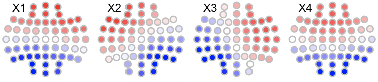
Example

Consider we have an unlabelled K=4 solution (in the text file k4) which we wish to label based on an existing set of K=4 templates (in the file t4), which are labelled with the canonical A, B, C and D labels.

We can visualize these using LunaR's convenience functions: in R, first the original maps (with arbitrary labels 1,2,3,4 (which R renames as X1, X2, X3 and X4 when reading columns with those headers):

library(luna)
k4 <- read.table("k4",header=T,stringsAsFactors=F)
par(mfrow=c(3,4),mar=c(0,0,0,0) )
for (i in 1:4) ltopo.rb( c = k4$CH , z = k4[,1+i] , mt = names(k4)[1+i])

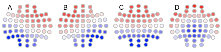
Likewise, the canonical maps are as follows:

t4 <- read.table("t4",header=T,stringsAsFactors=F)
for (i in 1:4) ltopo.rb( c = t4$CH , z = t4[,1+i] , mt = names(t4)[1+i])

To automatically assign labels using --label-maps:

luna --label-maps --options sol=k4 template=t6 new=k4.b th=0.8

 running LABEL-MAPS
  only assigning maps with spatial r >= 0.8 to matched template
  found 4 classes: A B C D
  read 4-class prototypes for 57 channels from t4
  found 4 classes: 1 2 3 4
  read 4-class prototypes for 57 channels from k4
   mapping [1] --> template [D] with R = 0.803188       
   mapping [2] --> template [B] with R = 0.991798       
   mapping [3] --> template [A] with R = 0.871168       
   mapping [4] --> template [C] with R = 0.990952

To plot the relabelled maps in n4:

n4 <- read.table("n4",header=T,stringsAsFactors=F)
for (i in 1:4) ltopo.rb( c = n4$CH , z = n4[,1+i] , mt = names(n4)[1+i])

Note that if we had required a more stringent matching, e.g. with `th=0.9 we'd see the following:

 mapping [1] --> template [D] with R = 0.803188 *** below threshold corr. -- assigning '?'
 mapping [2] --> template [B] with R = 0.991798       
 mapping [3] --> template [A] with R = 0.871168 *** below threshold corr. -- assigning '?'
 mapping [4] --> template [C] with R = 0.990952

and the fields would be not named:

CH      ?          B           ?           C
Fp1     1.33501    1.41774     0.194605    1.17416
Fp2     1.5269     0.895938    0.928289    1.10388
... etc ...

--correl-maps

Spatial correlations between maps

This convenience function reads a map from a file and prints the matrix of spatial correlations (between states) to standard output.

Note that this function does not require or accept an EDF or sample list.

Parameters

Option	Example	Description
`sol`	`k4.sol`	Read solution from file `k4.sol`

Output

Some notes to the console, and the matrix to standard output.

Example

If k4.sol is a file as output by MS (i.e. first column channels, subsequent columns are channel weights/loadings for each map, one per column):

CH      C           B           A             D
Fp1     1.33501     1.41774     0.194605      1.17416
Fp2     1.5269      0.895938    0.928289      1.10388
AF3     1.19466     1.34362     0.153383      1.2073
AF4     1.34935     0.625492    1.08554       1.11598
F7      0.833366    1.54421    -0.650062      0.78941
F5      0.880587    1.48185    -0.436373      0.966646
F3      0.868018    1.29965    -0.18313       1.09159
F1      0.913968    1.08758     0.185383      1.1776
... etc ...

To obtain the spatial correlation matrix:

luna --correl-maps --options sol=k4

In the console/log:

running CORREL-MAPS
  found 4 classes: C B A D
  read 4-class prototypes for 57 channels from k4

Written to standard output:

        C         B          A           D
C       1         0.608757   0.653712    0.892096
B       0.608757  1          0.216617    0.79893
A       0.653712  0.216617   1           0.401007
D       0.892096  0.79893    0.401007    1

Note the columns are kept in the same order as found in the input data.