Moonlight

In this final section, we'll repeat some (but not all) of the steps from the previous tutorial pages, using Moonlight instead of the command-line (lunaC) or R (lunaR) packages. As might be expected, this makes some things easier, but other things harder: that is the reason for both to exist, after all.

Moonlight: an interactive viewer, not a full analysis environment

Moonlight is an R/Shiny package wrapped around the Luna C/C++ library and the lunaR R package. It is intended to be an extended viewer for PSG signal data, with close bindings to some of Luna's functionality, e.g. for deriving hypnograms, for automated sleep staging, for spectral and other time-frequency analyses, for basic manipulations of datasets, and for embedding annotations alongside the signal data. It is expressly not intended to be a full analysis environment. For a start, Moonlight does not provide any mechanism for saving altered EDFs or annotation files. Although we currently allow arbitrary Luna commands to be evaluated, this is primarily provided for didactic purposes (i.e. as an immediate way to see Luna commands in action).

Display EDF files

If not already done, follow these initial steps to download the three tutorial EDF and annotation files. From there, you can upload one study at a time to Moonlight for viewing and other functions. There are several ways to run Moonlight, but the option that is (initially) easiest is to use our hosted version at http://remnrem.net/. Open that link in a new browser window (i.e. to keep this page also visible) and click on the Moonlight link when it appears to start a new session.

Restrictions on the number of concurrent Moonlight users at http://remnrem.net/

The http://remnrem.net is a free service - hosted by the Purcell lab and NSRR using the AWS cloud. As such, currently we necessarily have restrictions on the number of concurrent users this service is able to support. If the app gives a message that the maximum number of users has been reached, try again later. Alternatively, follow these instructions to use locally either a Dockerized version of Moonlight or install and run it directly using lunaR.

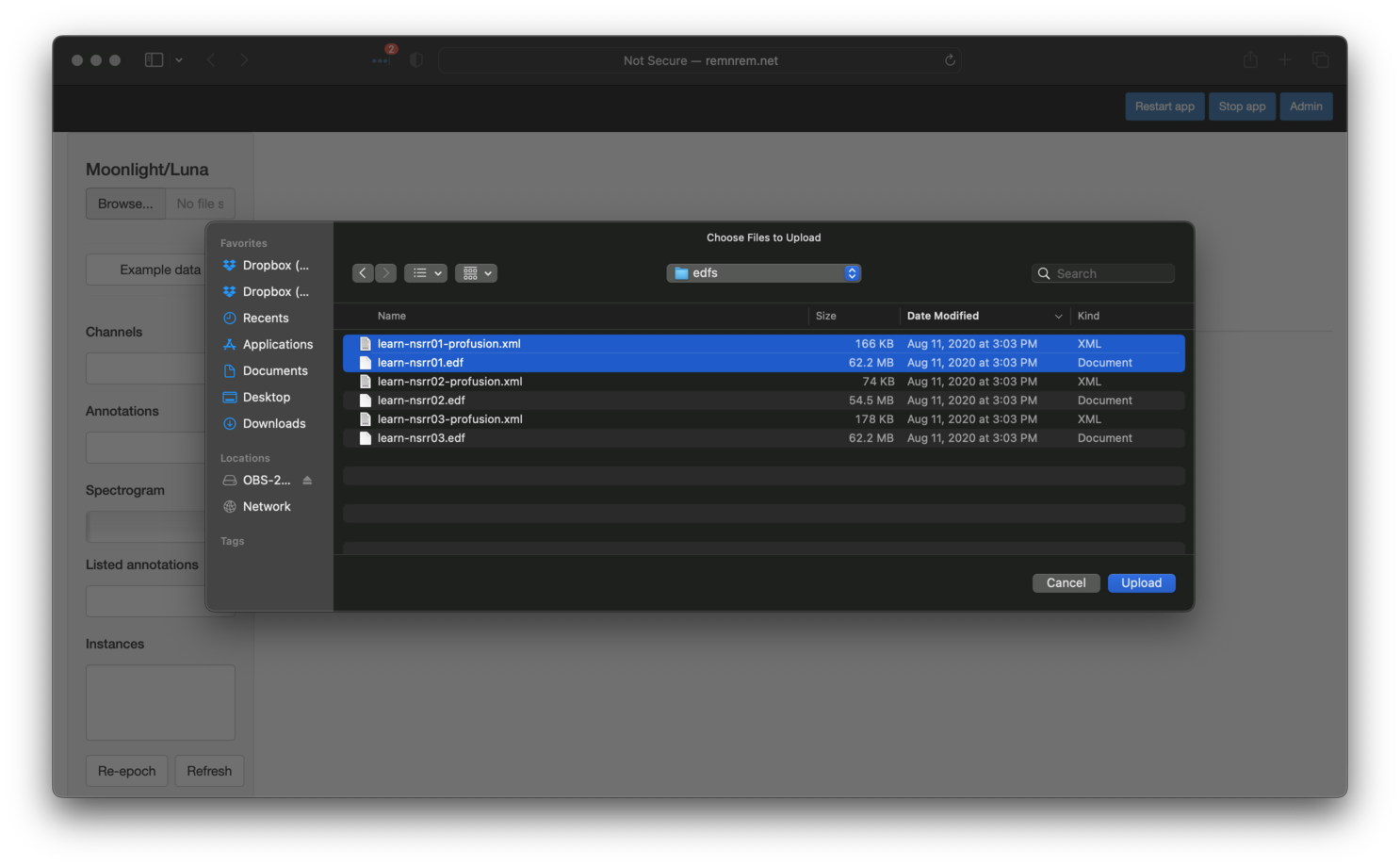
As described in the original tutorial (here), we used DESC and HEADERS commands to review the contents of each EDF and any associated annotations. This is easily achieved using Moonlight: once you have a running instance of the app, click the Browse button (top-left corner) and select the pair of EDF/annotation files (.edf and .xml) for individual nsrr01. Both files must be selected at the same time, and uploaded with a single click of the blue Upload button: i.e. it is not possible to load multiple files sequentially.

One EDF at a time

You can only view a single EDF at a time with Moonlight. You can upload multiple annotation files, but they are all assumed to be associated with the same, single EDF.

Running Moonlight locally

Faster uploads is another reason for installing Moonlight locally, especially if working with larger PSG files (e.g. hdEEG), or with datasets containing PHI that cannot be shared. (Note that absolutely no files or other derived data are stored on the server when using Moonlight, and we do not have access to any uploaded files).

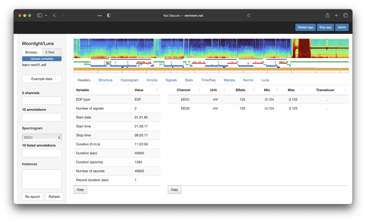
The upload may take 5 or so seconds depending on your connection. After upload has completed, you should see the following:

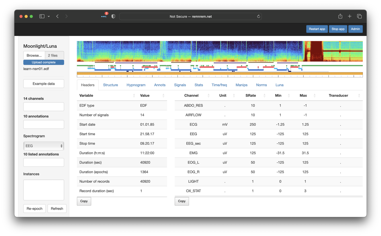
At the top of the page (and always present) is a spectrogram (generated by the PSD command), a hypnogram (generated by the HYPNO command) and a so-called mask bar plot (introduced below). Underneath, with the Headers tab selected, the lower panel shows two tables, with information primarily generated by the HEADERS command. These show the signals present and some other basic properties of the EDF, such as the length of the recording.

Channel/annotation alias/remapping

In the original tutorial, we used several options to specify channel lable aliases, that were applied on first loading new data. However, unlike command-line Luna, it is not possible to specify parameter files when uploading files to automatically remapping channel/annotation labels. In large part, such remapping is typically not necessary in the context of an single-dataset, interactive viewer. (Nonetheless, as shown below, it is possible to rename channels and remap annotations after upload, via some of the tools available in the Manips panel.)

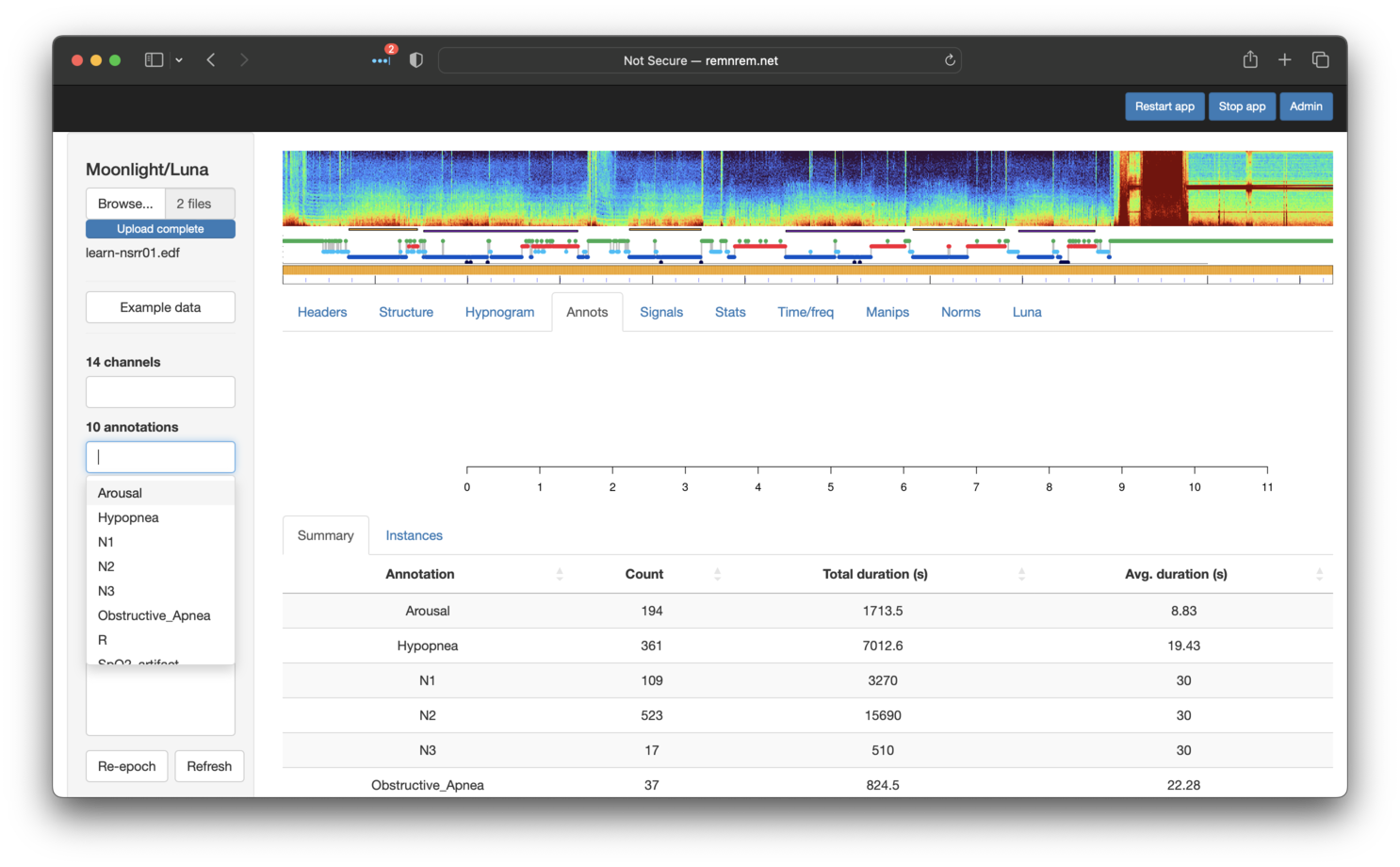
Moonlight also supports viewing associated annotations (e.g. from one or more XML, .annot or other files). As shown below, the annotations are also listed under the Annotations tab (fourth from the left). In this example, the list boxes in the leftmost panel show 14 channels (EDF signals) and 10 annotations:

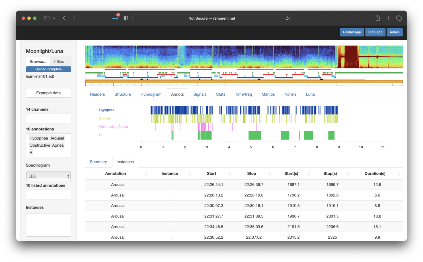
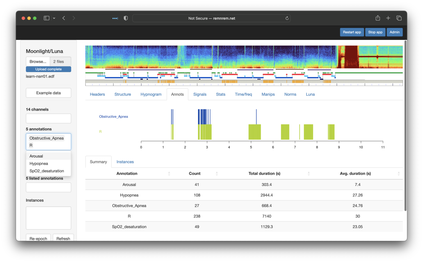
Selecting specific annotations in the left menu will display them in the Annotations tab: as shown below, here we have selected Hypopnea, Arousal, Obstructive_Apnea and R (REM sleep epochs). Note that the Annotations tab contains two sub-panels: Summary and Instances. Selecting the latter shows the specific events (with start/stop times) for the set of selected annotations (as shown below - the x-axis is hours from the EDF start). The Summary sub-panel (as shown in the image above) shows the number number and total duration for each class of annotation.

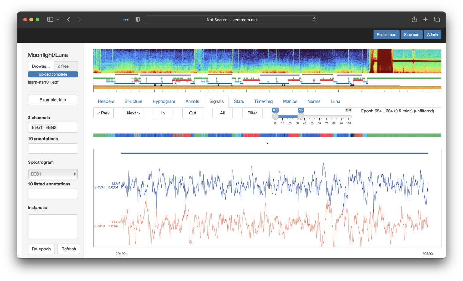
If channels (interchangeably referred to as signals here also) and/or annotations are selected in the left Channels and Annotations lists, the Signals tab (fifth from the left) will show a plot of the raw signals. By default, this is centered on a 30-second window, but can be expanded by clicking on Out (or All). If too long an area is selected, Moonlight will not show the signals, as this could involve plotting millions and millions of datapoints (any selected annotations will still be shown, however).

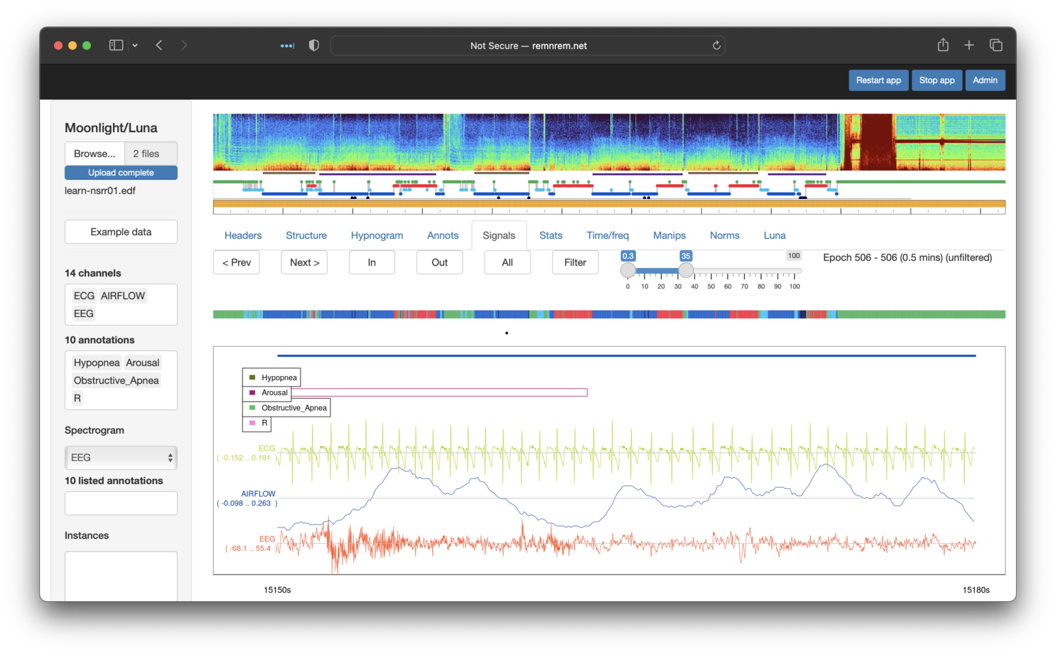
Note the reduced hypnogram just above the signal plots, with color-coded bars indicating wake, NREM or REM epochs as green, blue or red respectively. The black dot below it represents the currently displayed epoch(s) of raw signal(s) in the main portion of the window. Clicking on this bar moves the viewer to that position; the Prev and Next buttons can also be used to shift the viewing window backwards and forwards in time.

Signal summary statistics

The next step of the original tutorial, as described here, was to estimate some basic statistics for various channels - e.g. starting with the SaO2 channel. We can repeat that process by simply visiting the Stats tab and selecting SaO2 in the left Channels list:

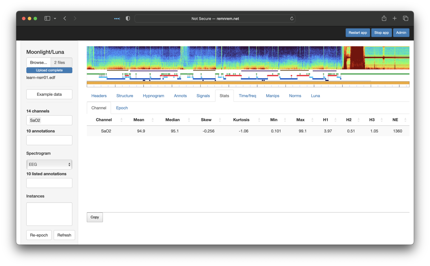
The table shows some of the whole-night statistics for this channel, calculated on-the-fly and, as such, respecting any masks that are set, as shown below. Clicking on the Epoch sub-panel shows epoch-level equivalent metrics (not shown).

Channel-wise versus epoch-wise statistics

If you look carefully, you'll see the original tutorial gave different means compared to these. This reflects the fact that the Stats module runs STATS epoch rather than simply STATS as per the original tutorial. The epoch argument means that Luna estimates overall statistics (e.g. mean) as the median of all epoch-level means (as well as generating/reporting epoch-level statistics). That is, the values reported by Moonlight reflect MEDIAN.MEAN from STATS epoch output, rather than MEAN.

Working with annotations

We've seen above how the Annotations tab provides a summary and tabulation of all annotations. We've further seen how annotations can be integrated into the Signals viewer.

As an additional check of the correspondence between what we saw in the tutorial and what we see via Moonlight, consider that the first individual (nsrr01) had 37 Obstructive_Apnea events. Indeed, from the screenshot shown in the prior section, we saw this was also the case here.

The next step in the tutorial asked how many events were observed during REM sleep (N=27). We can repeat this in Moonlight by taking advantage of the fact that the Annotations tab respects any masks currently set. We can apply masks by going to the Manips (manipulations) tab, and selecting the Mask sub-tab. A box lists the available annotations that can be used to either include or exclude epochs. This feature is a simple wrapper around Luna's MASK command, so be sure to review the details there.

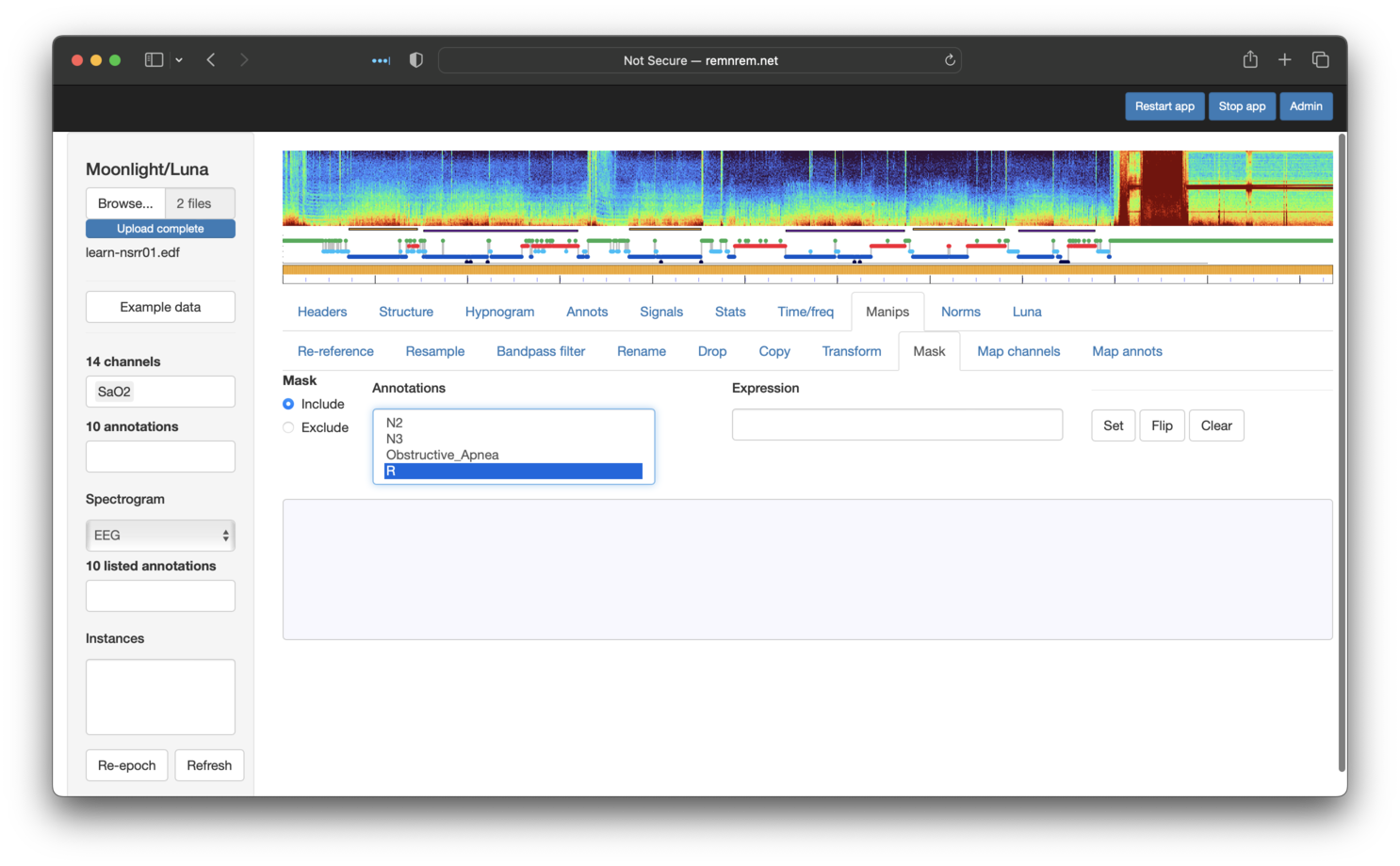
The options above equate to

 MASK ifnot=R

Note that the Expression box should be left empty if selecting annotation(s) from the list -- this box provides a means for adding different options to MASK (as we see below when using the hms flag).

After clicking Set, you should see the following:

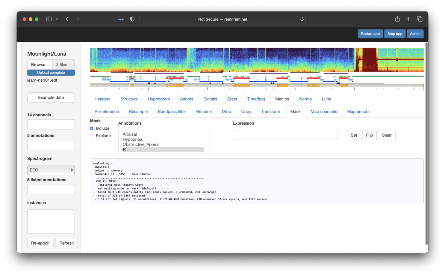
Note that the bar underneath the top hypnogram is now striped gray and orange. Gray means that the mask has been set for that epoch -- whether or not a mask has been set corresponds to whether or not that epoch is REM sleep (red in the hypnogram) or not.

If we go back to the Annotations panel and select Obstructive_Apnea and R (REM), you'll see that only apnea events that fall in REM are now shown:

An additional nuance covered in the original tutorial was to change the definition of overlap, to restrict to only counting events that started in a REM epoch (rather than the default of including all annotations with any overlap. Reflecting an inevitable trade-off between simplicity and flexibility, the Annotations panel does not support this additional option directly.

However, here we take this as an opportunity to see how the Luna panel (an advanced feature) allows us to recapitulate almost any Luna command within Moonlight. As pictured below, this panel allows an arbitrary series of Luna commands to be evaluated. To mimic the behavior of ANNOTS start in the original tutorial, we can type it in here and then click Execute:

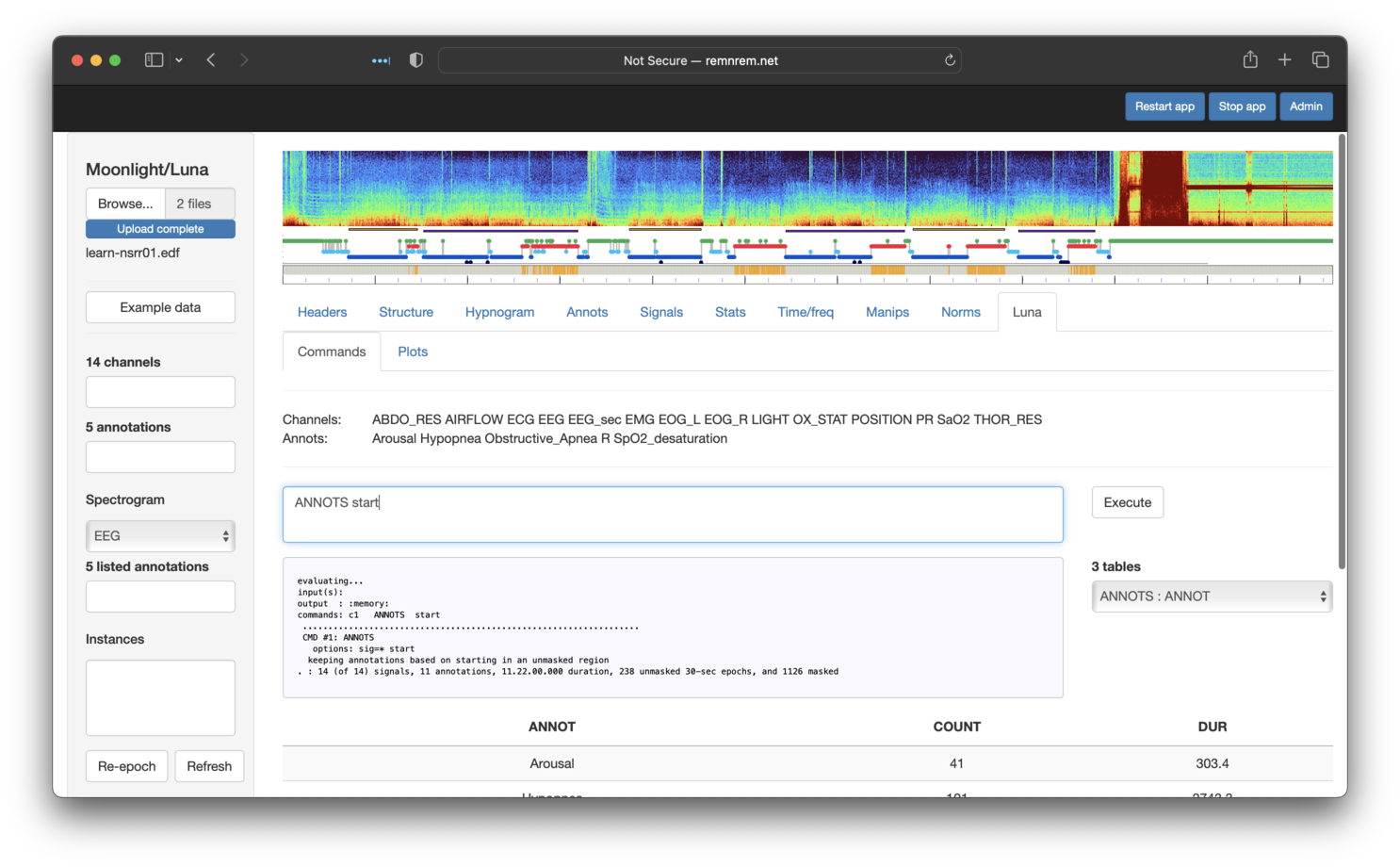
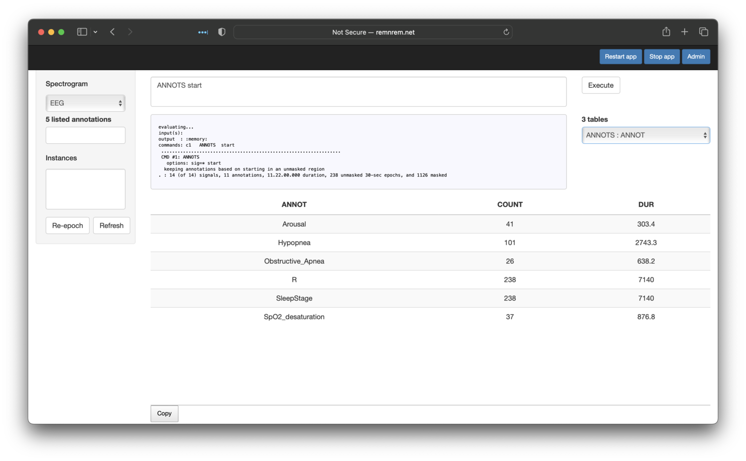
If the evaluated command(s) generates output tables (i.e. as described here, these will be listed below the Execute button. The bottom table shows the currently selected table from this list: here output from ANNOTS stratified by ANNOT (annotation class). Here we see that there are 26 Obstructive_Apnea events under this definition (i.e. starting in REM), which matches the original Luna tutorial.

We can alternatively select the table that lists all individual events (starting in REM), as shown below:

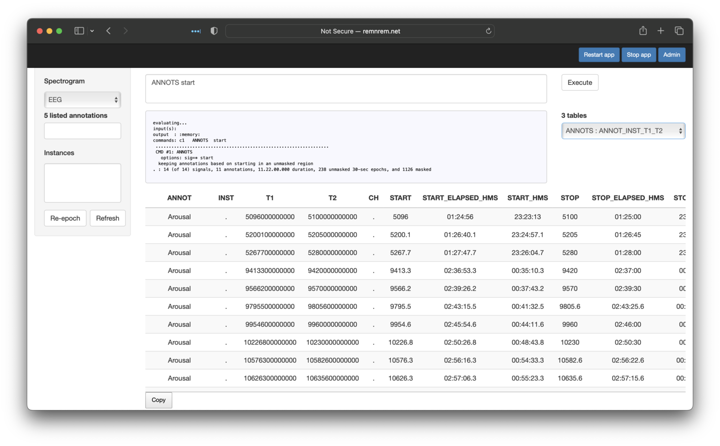
Note that, as with most Moonlight panels, these tables have a Copy button underneath - if clicked, the contents of that table are copied to the Clipboard, and can then be pasted into a program such as Excel or otherwise saved to a text file.

Hypnograms

As shown above, if sleep stage annotations are recognized by Luna (they will be mapped to the canonical forms N1, N2, N3, R and W, as well as ? and L), Moonlight will draw a hypnogram under the spectrogram when first attaching the new dataset. The Hypnogram tab (third from left) allows one to look at hypnogram-derived metrics in Moonlight, including stage durations.

In the original tutorial we saw that the first individual had 54.5, 261.5, 8.5 and 119 minutes of N1, N2, N3 and R respectively. Selecting the Hypnogram/Stages sub-panel, we see the same information (along with some additional metrics):

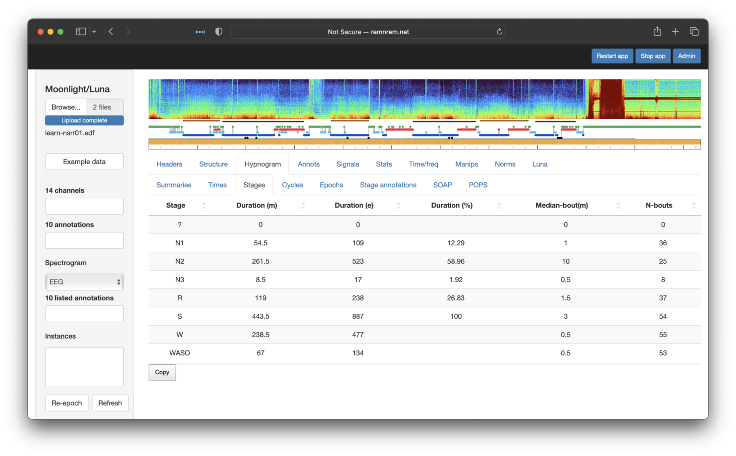
Information on sleep cycles and epoch-level descriptions are also available via the other Hypnogram sub-panels.

Epoch-level masks

To see how Luna masks are applied, it can be useful to use Moonlight to check that are doing what we assume they should: To this end, we will reproduce these steps from the orignal tutorial, which involved selecting epochs for the first individual that:

• were in persistent sleep (at least 10 minutes of sleep prior)

• occured between 11pm and 3am

• were during stage 2 NREM sleep

• did not contain any apnea or hypopnea events

Hint

As noted above, Moonlight is not the ideal platform for implementing multi-step analyses - if for no other reason, this type of GUI fundamentally violates the principles of reproducible research.

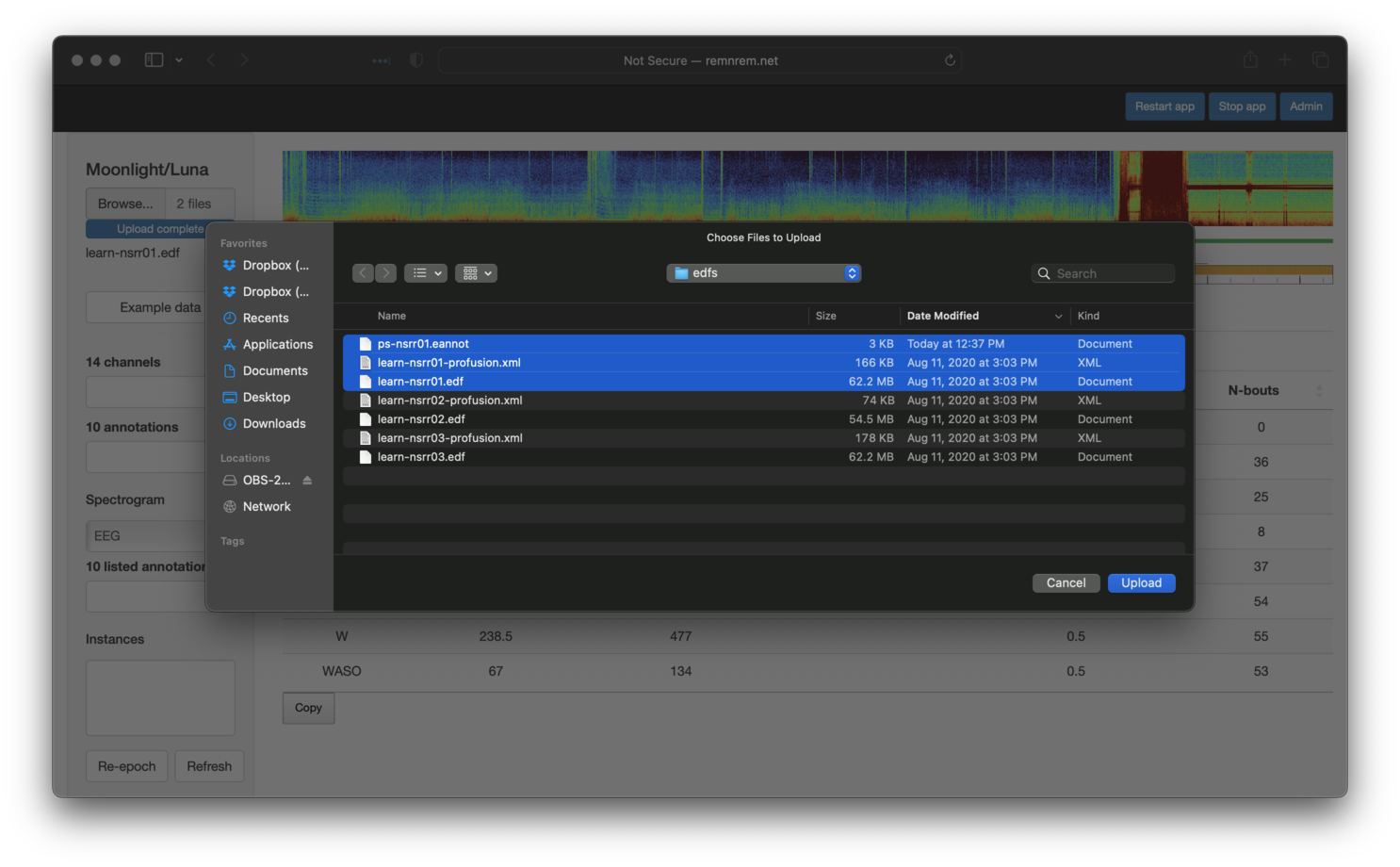
In the original tutorial we created an intermediate file to flag epochs in persistent sleep (named ps-nsrr01.eannot). We can attach such .eannot format files (here, a simple file of one line per epoch, one label per line: here PS0 or PS1), by additionally selecting it when first uploading the EDF. To do this, we need to reload the two original files (EDF and XML) alongside this new annotation file. (Moonlight primarily recognizes (NSRR format) XML, .annot and .eannot files as annotation files.) One current limitation is that all files must be in the same folder in order to be selected for upload, and so we'll copy ps-nrr01.eannot into the edfs/ folder (see the original tutorial for how this file was created - it is also present under the cmd/ folder in tutorial.zip).

Re-uploading these three files (note: it is not necessary to have nsrr01 as part of the filename - all files attached at this step will be assumed to be associated with the same, single EDF):

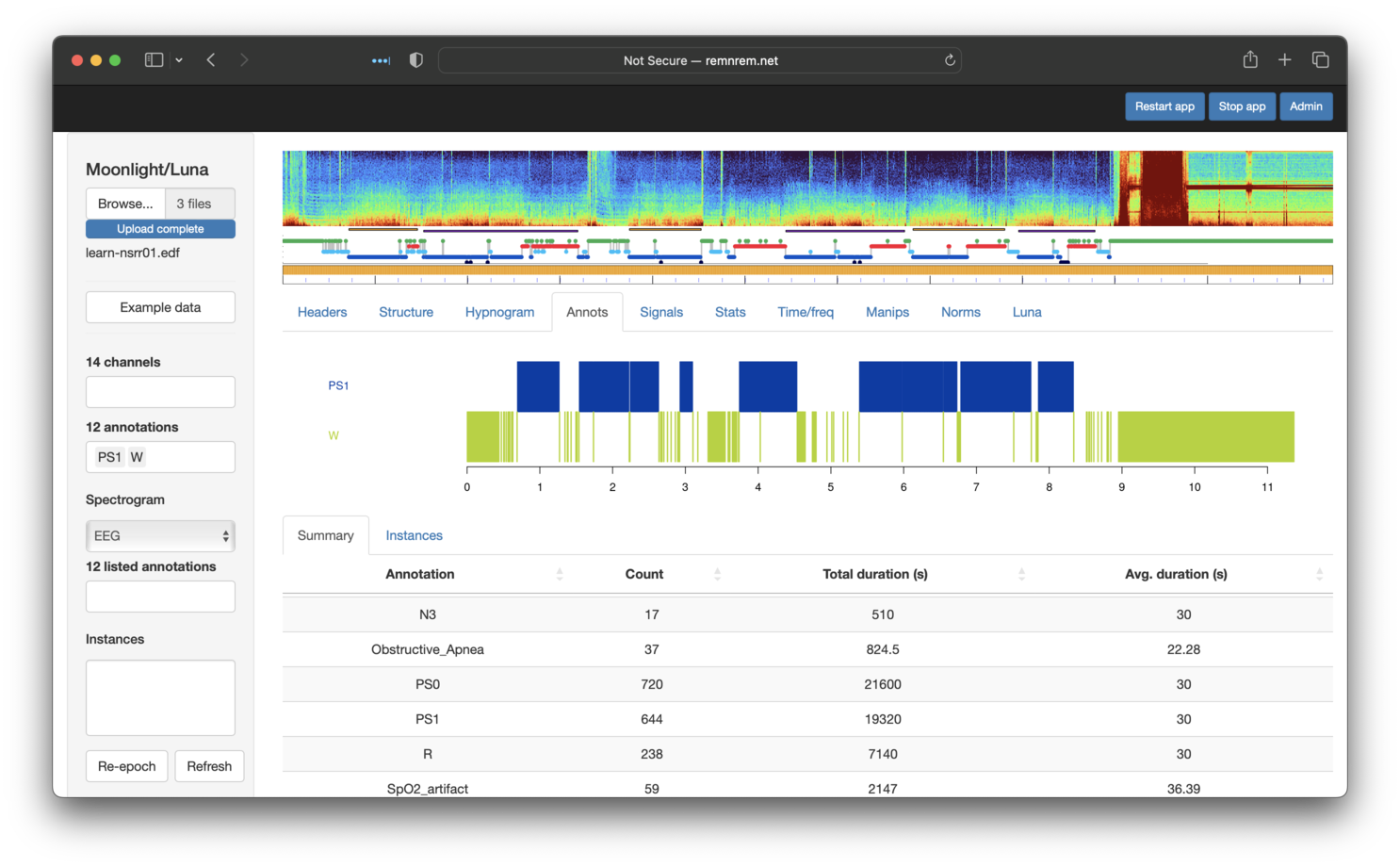
We can now view the new PS1 annotations alongside wake (W) epochs - as expected, no W epochs are PS1, but not all sleep epochs are PS1, as per the definition of persistent sleep used here:

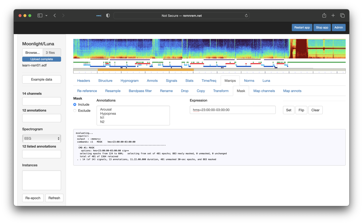
To follow the steps of the original tutorial (which we'll do in the same order - although they could be performed in any order), we'll first restrict to epochs between 11pm and 3am. This involves using the hms option as part of a mask (under the Manips tab in Moonlight). Note that the syntax is the same as the original Luna commands. After clicking Set, you should see that the mask plot bar (under the top hypnogram) nows shows that only epochs in this particular 4 hour interval are included (colored orange, rather than gray):

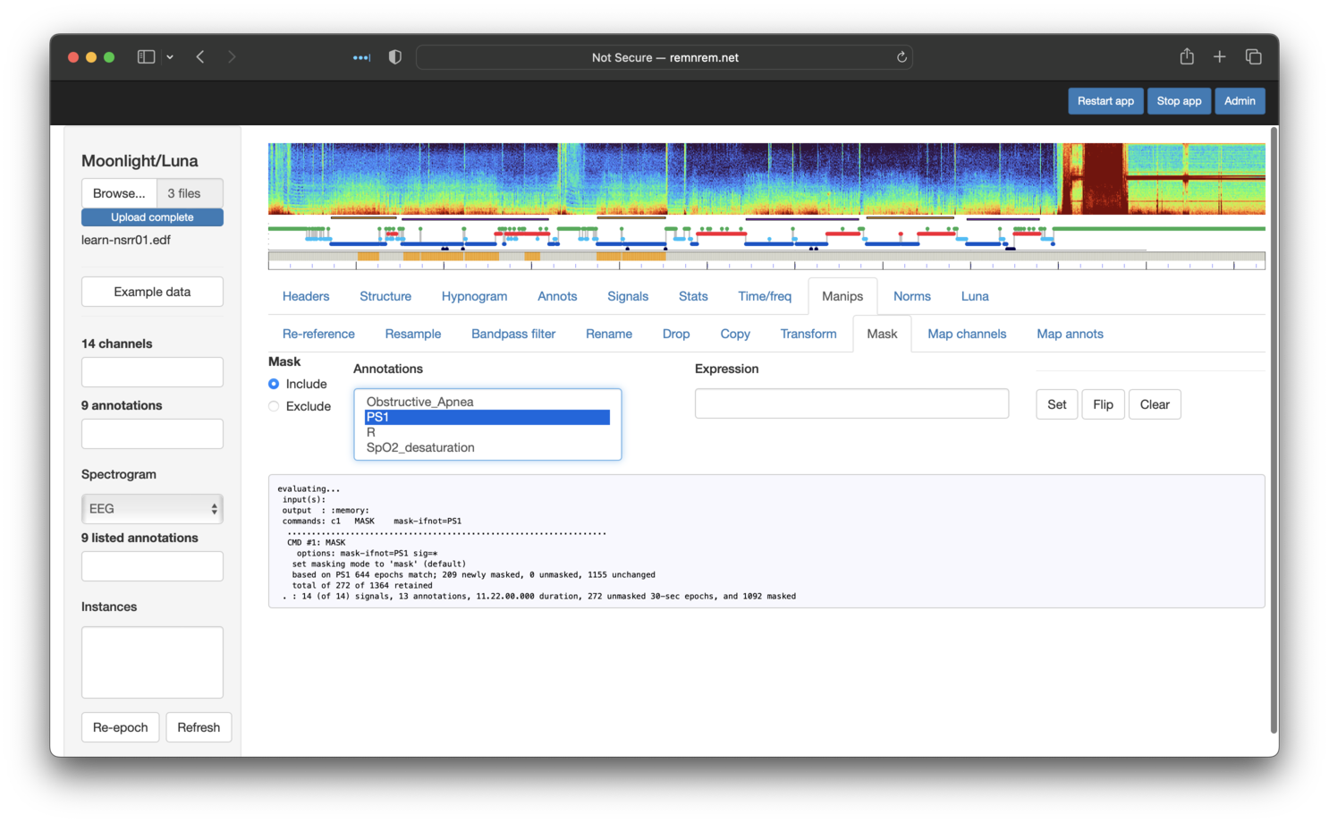
To next restrict to persistent sleep PS1 epochs only, we can use the same Mask panel, but selecting to Include PS1 epochs. (We could equivalently have selected to Exclude PS0 epochs). This has the effect of further graying-out certain epochs in the mask plot bar:

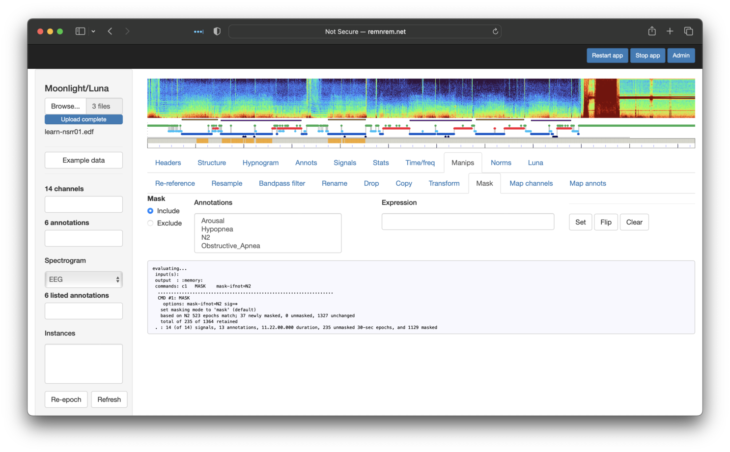
Next, we restrict to N2 only, using a similar approach. After this step, we'll see the following:

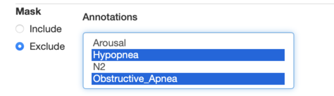
Finally, we'll exclude any epochs that have either an overlapping Obstructive_Apnea or Hypopnea event. You can select multiple annotations to exclude by holding down shift or control when selecting:

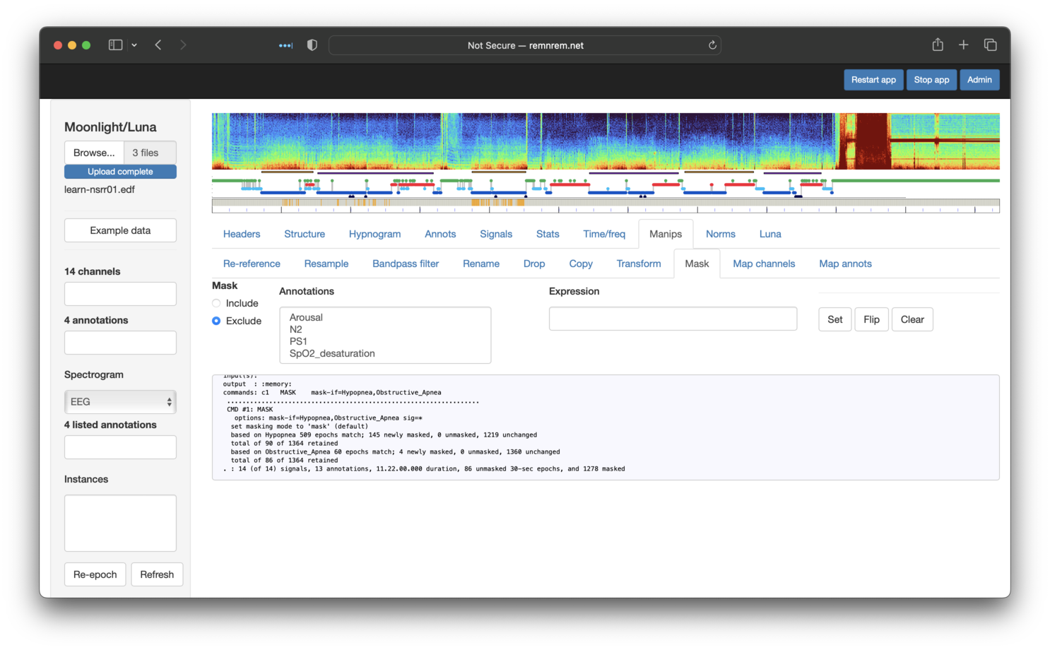
Then clicking on Set should remove (more precisely, set the mask flag for) those epochs too. The small gray box that shows the console output from Luna shows (final row) that we are left with 86 remaining epochs, which matches the original tutorial:

Having set this mask, we can restructure the internal dataset, to actually remove masked epochs rather than just flagging them. This leaves us with what is effectively a discontinuous (EDF+D) in-memory dataset. Restructuring can be achieved by clicking Re-epoch in the lower left corner of the screen. Now the previously gray epochs (i.e. with a mask set but not removed) will be now be white (i.e. actually removed from the in-memory dataset). The Structure/Segments tab (second from the left) shows the structure of what is now a discontinuous recording/EDF+D:

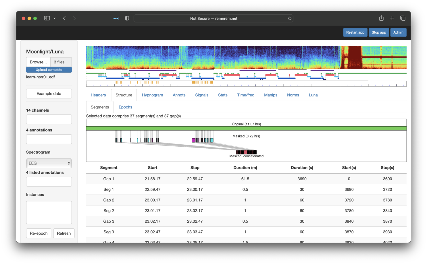
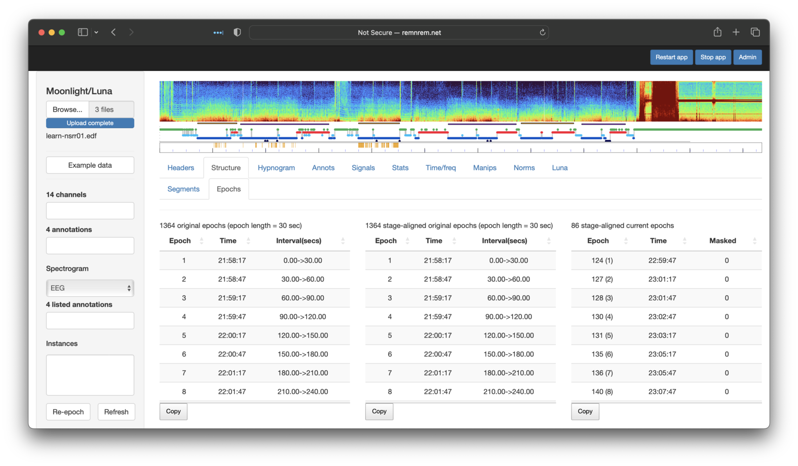
That is, from the original recording, we selected (86/2)/60 = 0.72 hours of sleep. The table below the cartoon also shows where the segments/gaps start/stop. Selecting the adjavent Structure/Epoch sub-panel shows three breakdowns of epochs:

• leftmost: original epochs (30 seconds by default) starting from the start of the EDF (for a continuous recording)

• middle: epochs aligned with any sleep stage annotations - this may be different from the previous if sleep staging is not aligned with the start of the recording, e.g. the first staging annotation starts 28 minutes and 2 seconds into the recording, but for many datasets these will be identical to the left table

• rightmost: the set of aligned epochs in the current in-memory dataset, i.e. following any masking/restructuring - here we see there are 86 epochs as expected. The numbers in brackets show the epoch count in the revised dataset (i.e. the first epoch in the extracted dataset was the 124th epoch in the original, etc).

To summarize, with the above steps we have recapitulated the following Luna commands, as per the original tutorial:

EPOCH
MASK none
MASK hms=23:00:00-03:00:00
EPOCH-ANNOT file=cmd/ps-nsrr01.eannot
MASK mask-if=PS0
MASK mask-ifnot=N2
MASK mask-if=Obstructive_Apena,Hypopnea
DUMP-MASK
RE

Manipulating EDFs

The next section of the original tutorial showed some examples of manipulating signals: e.g. changing physical units for EEGs, resampling, filtering and re-referencing. Although Moonlight is not the obvious tool for making such changes (i.e. given that you cannot save/download EDFs), inasmuch as it might be useful for certain viewing procedures (or as a prelude to automated staging), the Manips panel gives a selection of sub-panels to perform these steps. Each is a trivial wrapper around an underlying Luna command, and so you should consult the appropriate Luna documentation as needed:

Moonlight panel	Luna command	Description
Re-reference	REFERENCE	Offline rereferencing one or more signals against a single reference
Resample	RESAMPLE	Resample one or more signals
Bandpass filter	FILTER	Apply bandpass filter
Rename	RENAME	Rename a single signal to something else
Drop	SIGNALS drop	Remove one or more signals from the EDF
Copy	COPY	Generate a copy of a single signal
Transform	TRANS	Arbitrary transformations of signals
Mask	MASK	Set the epoch mask given various criteria
Map channels	CANONICAL	Make new channels with specified labels/convntions
Map annots	REMAP	Change annotation labels

For example, to follow the (quite arbitrary) steps of the tutorial:

• extratct two central EEGs only, and rename them as EEG1 and EEG2

• change physical units to milli-volts

• resample to 100 Hz

• bandpass filter to 0.3 - 35 Hz

• re-reference EEG1 against EEG2

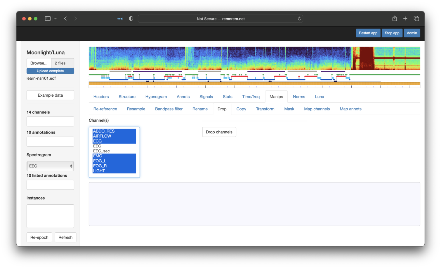
We first use Drop, selecting all channels except the EEGs:

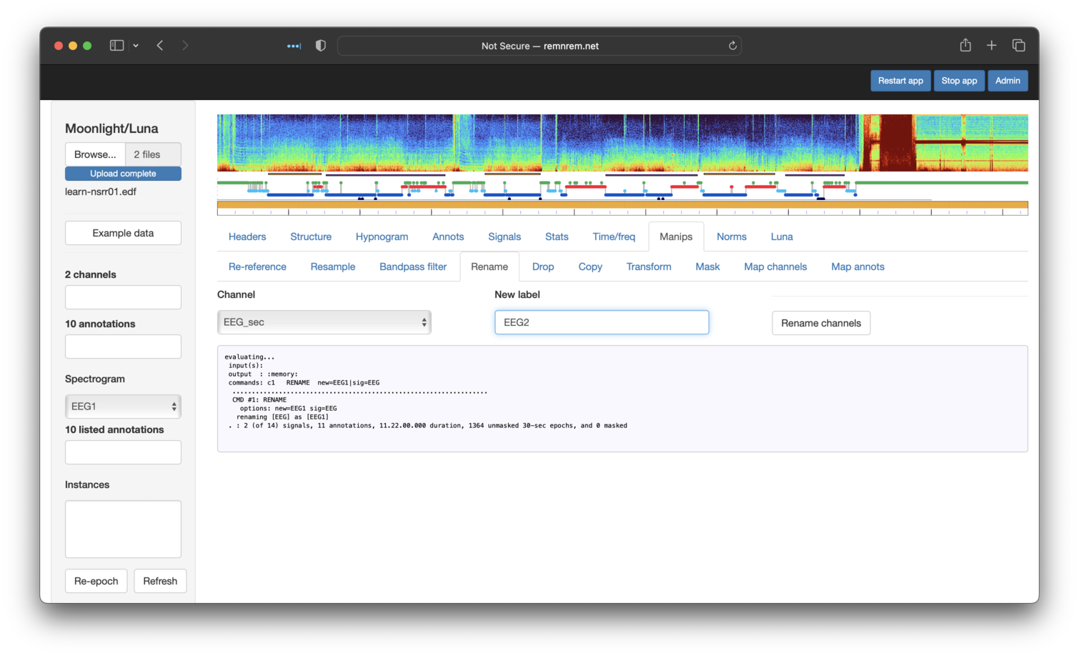
We then use Rename to set the labels to EEG1 and EEG2 (having to repeat this step for each):

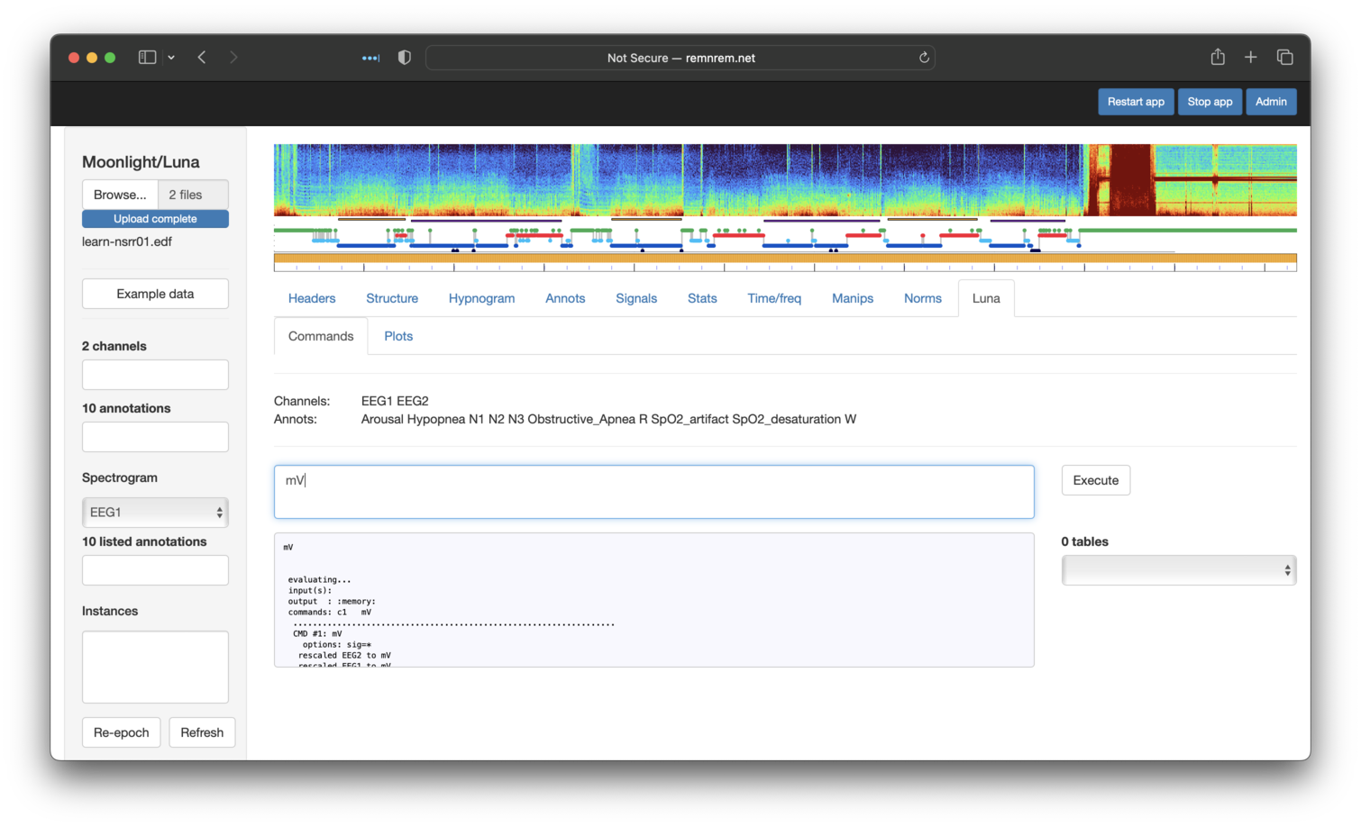
There is no Manips tab to change units per se, but we can use the Luna tab to apply the simple mV command (no sig is needed here, as we've already dropped all channels except the two EEGs, i.e. so mV will be applied to both):

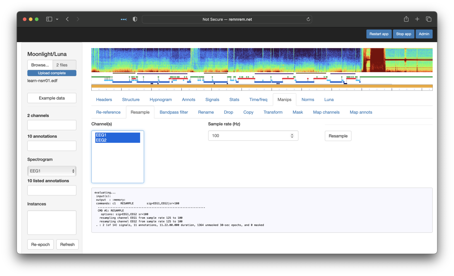
Next, the Resample tab (selecting both signals) to get 100 Hz signals:

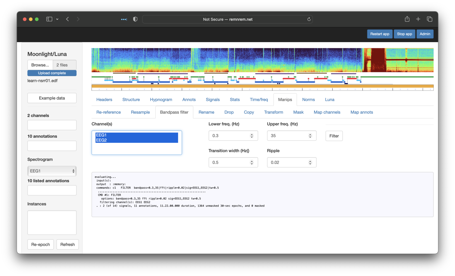
Next, applying a bandpass filter to both EEGs:

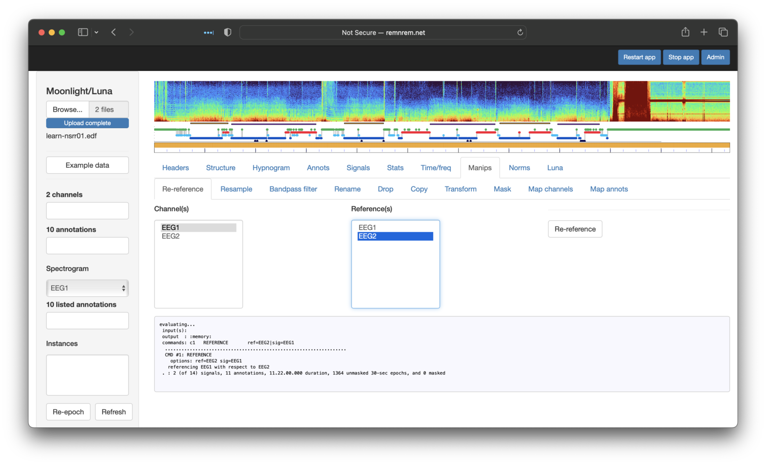
And finally, re-referencing EEG1 against EEG2 (this is just to illustrate the options available -- i.e. referencing two central, contralateral-mastoid referenced channels against each other is not likely to be a meaningful operation in practice):

Having performed these steps, returning to the original Headers table, it should have updated to reflect these changes: i.e. it now just lists two signals (EEG1 and EEG2) that have mV units (previously uV), etc.

We can also view these newly transformed signals as we would original signals.

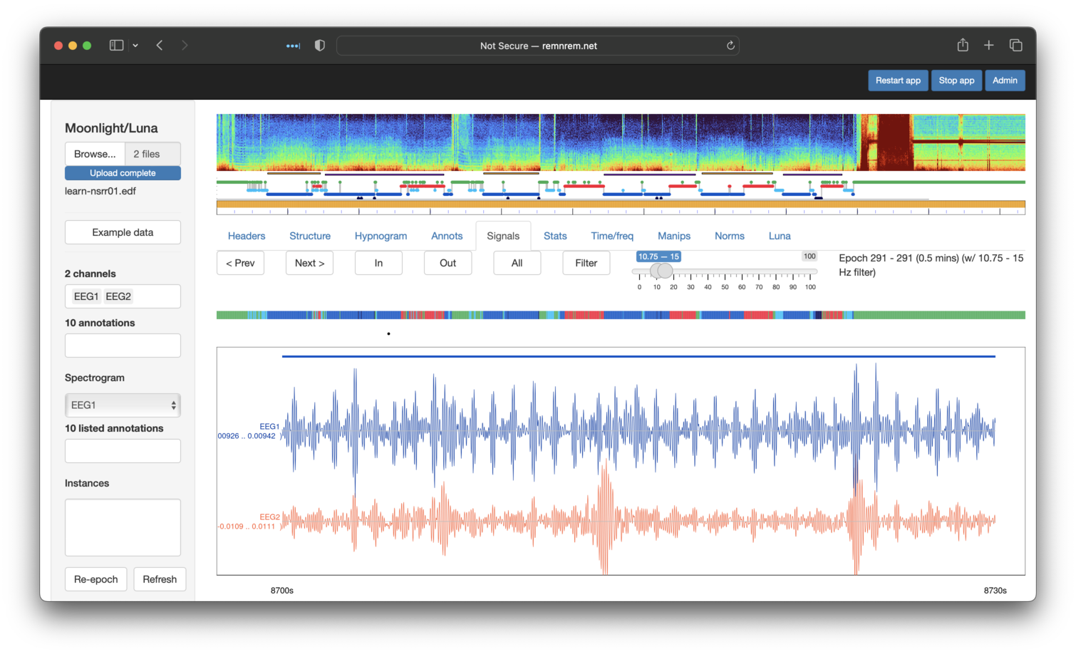
Finally, when viewing we can apply on-the-fly bandpass filters to the signals also - by selecting the desired frequency range and then clicking Filter (to toggle it on/off). With the two EEGs filtered in the sigma range, we see a clear periodic pattern (sigma power bursts approximately every second in quite a regular manner), particularly for EEG1 which is likely artifact (as will be explored in the next section). This visualization shows that clear value of visalizing signals.

Artifact detection

Note

Again, this example is presented with the caveat that the command-line Luna is a far superior tool for real data analysis. Here we present this for didactic value and to mirror the original Luna tutorial, in which we apply some very simple artifact detection approaches. Luna has a broader range of artifact detection and correction methods than is covered here, as described on this page

The steps of the original tutorial basically ran through the following commands (in cmd/sixth.txt):

EPOCH 
MASK if=W
RESTRUCTURE
FILTER bandpass=0.3,35 ripple=0.02 tw=1
ARTIFACTS mask
CHEP-MASK ep-th=3,3,3 epoch
CHEP epochs
DUMP-MASK

After first clicking Refresh (lower left panel) to clear any existing masks, etc, for the attached nsrr01 EDF, we can directly paste the above multi-step Luna script into the Luna panel, and select Execute (note - the panel scrolls, so not all lines are shown here):

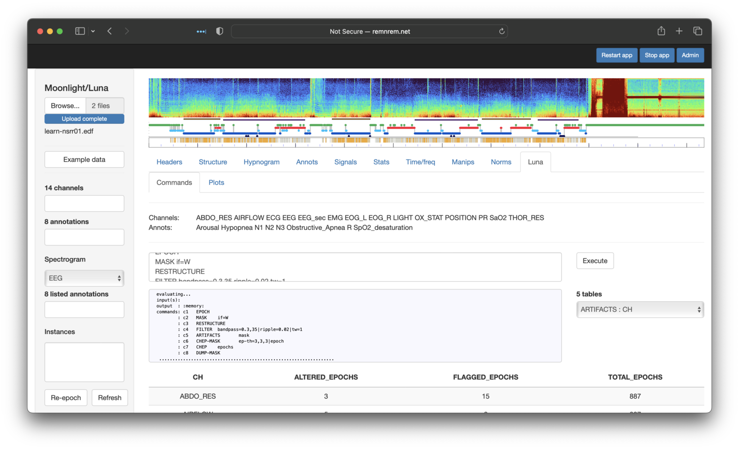
This produces all of the same output as the orignal Luna run, which is accessible via the Tables embedded in this page. Here we see that five tables have been generated. By default, the first is automatically selected and shown: in this case, output from ARTIFACTS stratified by CH (channel):

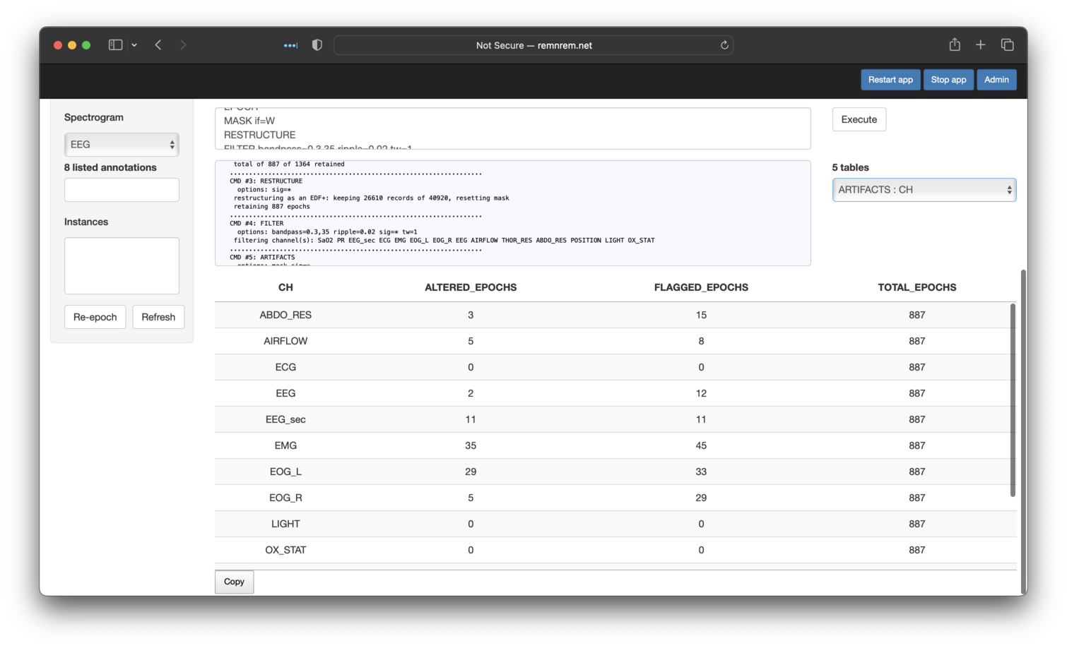
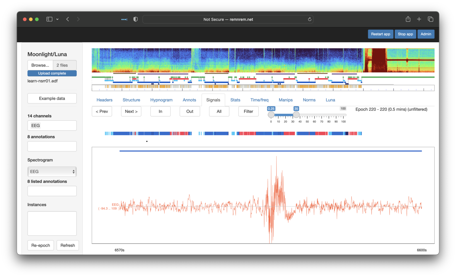
Looking at the other tables present, we can see that the DUMP-MASK command flags the mask epochs (not shown here). As in the orignal tutorial, we flagged a particular epoch (220) for visual review. Indeed, if we look at the DUMP-MASK outputs, we'd see that epoch 220 is indeed flagged as an artifact. We can then directly use the viewer to look at this signal - i.e. giving the same view of the original tutorial:

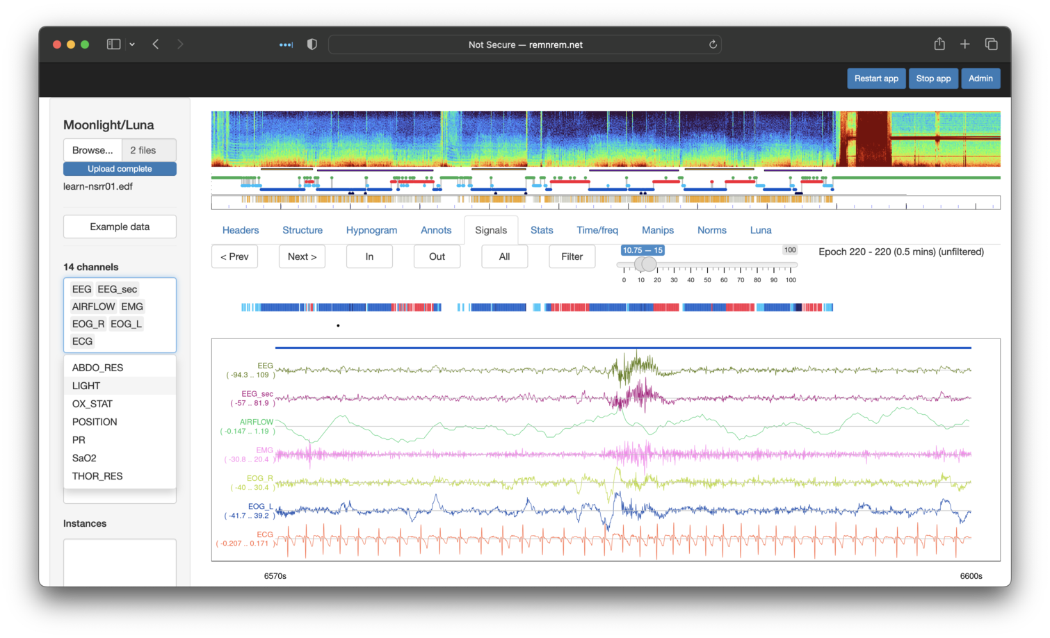
Naturally, one advantage of using an explicit viewer like Moonlight is that it is easier to click on other channels to see the broad picture of what happens during this epoch:

Spectral/spindle analyses

Note

At the risk of repeating this one time too many: Moonlight is absolutely not the optimal platform for full-blown analyses of sleep data - the command-line Luna is the preferred tool in that case. With that aside, here we will repeat the final steps of the tutorial using Moonlight.

Finally, the original tutorial performed some limited spectral and NREM spindle analyses of the sleep EEG. There is no single interface panel for this - rather, we will use the Luna panel to evaluate arbitrary Luna commands - here the (slightly modified) text from cmd/seventh.txt:

SIGNALS keep=EEG 
EPOCH 
MASK ifnot=N2
RESTRUCTURE
FILTER bandpass=0.3,35 ripple=0.02 tw=1 fft
ARTIFACTS mask
CHEP-MASK ep-th=3,3,3
CHEP epoch
RESTRUCTURE
PSD spectrum dB
SPINDLES fc=11,15 annot=spindles per-spindle

After copy-and-pasting the above into the appropriate place [which reads (Enter Luna commands here)] and clicking Execute, you should see the following (assuming nsrr01 was uploaded and/or you pressed Refresh after doing earlier exercises):

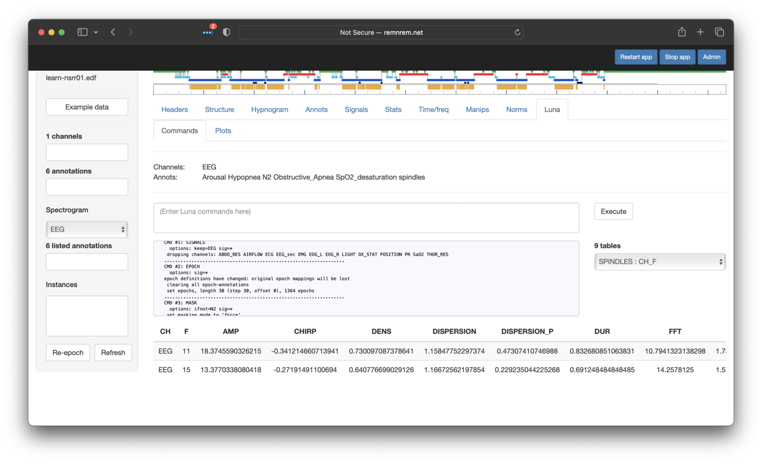
That is, as per the standard output for Luna, we see the CH x F table of the SPINDLES command (described here. For example for the EEG channel, we see the density (DENS) of both fast and slow spindles is quite low (<1 spindle per minute). Other metrics are scrolled off the right side of the screen (you can scroll across the table with the mouse).

Displaying Luna tables

Unlike other parts of Moonlight, where it know the structure of the expected output and can easily format it nicely, the Luna tab generates arbitary tables in terms of the columns, rows and header labels. As such, it is not as straightforward to automatically format items for neat display.

Because we added the annot=spindles flag to SPINDLES it generated an annotation to indicate when the detected spindle events occurred. These will be automatically added to the lists of available annotations, and can be viewed in the Signals tab along with other signals and annotations:

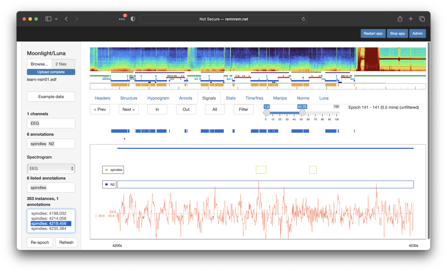
Note that we've selected the spindles annotation in both the top Annotations box (which controls which annotations are displayed) and the lower Listed Annotations also. The latter box then lists the individual events in the box below (lower left pabel). Clicking on an event will move the Signals window to that position. Note that spindles must also be selected in the top box in order to see it in the display. You can zoom into the main display by selecting the desired area with the mouse, e.g. to see the spindle close up (not shown). To get back to the original view, perform a single-click anywhere in the display window.

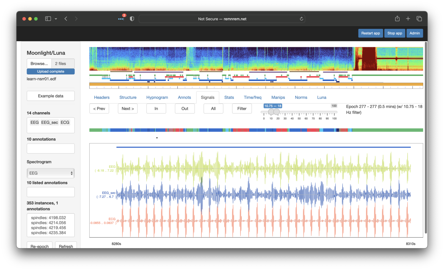
As a final step (which goes beyond the original tutorial but underscores the value of visual analysis), we'll revisit the issue of potential artificat in the EEG (EEG1) signal as noted above. If we turn on the Filter set to the approximate sigma range (here 10.75 Hz - 18 Hz) and also add the ECG channel to the display also, we can see a clear correspondence between spikes in the EEGs and the ECGs:

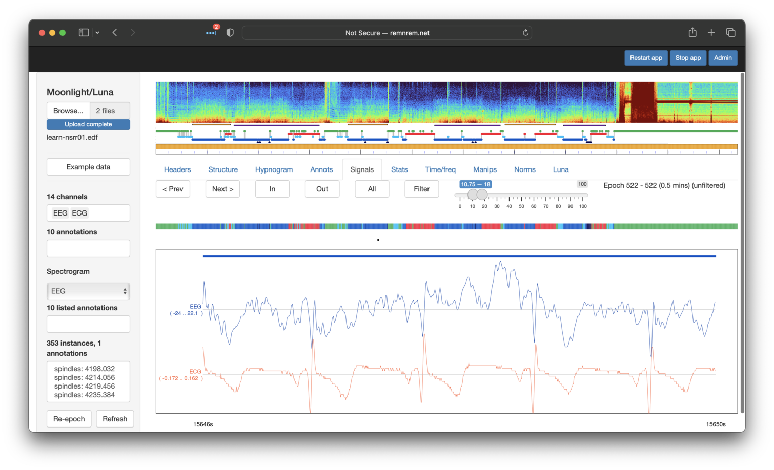
Looking at the raw traces (toggling Filter off) and zooming into (by selecting a region of the main view panel with the mouse) we can see a clear correspondence between the QRS complex R peak in the ECG and what is seen in the EEG (here just showing one EEG channel). This is a classic case of cardiac contamination in the EEG signal.

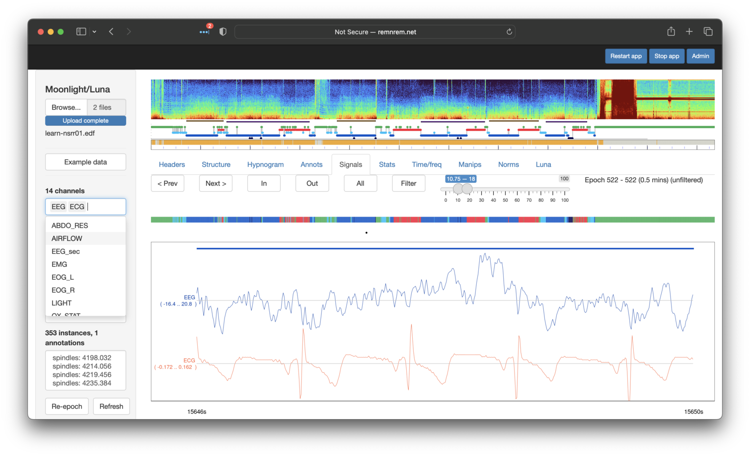
We can attempt to attenuate this contamination with Luna's SUPPRESS-ECG command, i.e. running the following via the Luna tab in Moonlight (not shown):

SUPPRESS-ECG ecg=ECG sig=EEG

After performing the above and returning to the same region in the Signals tab, we can see the artifact has been greatly (if perhaps not completely) removed:

Although beyond the scope of this tutorial, if one re-runs the `SPINDLES command on the signals after dealing with cardiac contamination effects, we typically see increased spindle density estimates (as the cardiac contamination has the effect of increasing baseline sigma activity, making it harder to detect spindles above the increased noise).

---

This concludes the Moonlight tutorial, seeded on the original Luna (and lunaR) tutorials. Moonlight has a number of other capabilities not even mentioned here. To learn about these other features (including automated sleep staging) please visit this page.