Evaluating, manipulating & predicting stages (SOAP/POPS)
In this vignette, we demonstrate using Luna to evaluate, manipulate and predict sleep stages, via the SOAP and POPS family of commands.
Single- and multi-channel methods
For simplicity, here we focus only on a single EEG channel (C4-M1). However, all methods described here can be straightforwardly applied in a multi-channel EEG context, as well as including other types of channel, e.g. EOG, EMG, etc.
Data
To illustrate these methods, we'll focus on a single recording: one individual from the Sleep Heart Health Study, which is available via the NSRR. These signal data come with a manually-scored hypnogram: 30-second epochs scored following AASM guidelines (i.e. based on the EEG, EOG and EMG). After downloading the EDF and its associated XML, we first create a sample list (albeit here, for only one sample):
luna --build -nsrr . > s.lst
s.lst, linking EDF, annotations and ID (here coded as shhs1-0000)
shhs1-0000 ./shhs1-0000.edf ./shhs1-0000-nsrr.xml
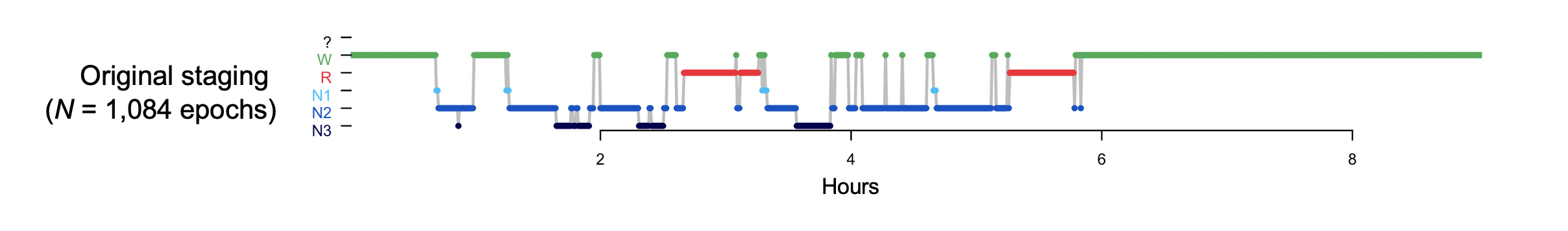
We can view the manually-scored hypnogram using the R lhypno()
function in LunaR:
library(luna)
sl <- lsl( "s.lst" )
lattach( sl , 1 )
shhs1-0000 : 5 (of 5) signals, 10 annotations, 09.02.00.000 duration
Via lunaR, we can call the HYPNO command to get a table of stages by epoch:
k <- leval( "HYPNO epoch" )
lhypno():
lhypno( k$HYPNO$E$STAGE )
Evaluating overall staging quality
The above hypnogram above looks quite reasonable, albeit with a relatively short sleep duration, i.e. TST is under five hours. Although there are only two complete NREM cycles, we see a typical hypnogram structure, with cycles containing relatively more N3 sleep earlier in the night, and more REM sleep later on.
But, can we be more sure that it is in fact consistent with the signal data and accurately reflects the night's sleep? At an extreme, the staging (or signal) data may have been corrupted or - especially in the context of a study involving thousands of people - even mislabelled on exporting, such that there is now no correspondence between signals and staging files. Alternatively, the staging may simply be of very low quality/consistency.
The SOAP command (Single Observation
Accuracies and Probabilities) can partially address this type of scenario. In
short, it takes as inputs one or more signals, as well as a set of "observed"
stages. These will typically be for 30-second epochs staged manually, but
this need not be the case (e.g. they could be from some other automated predictor.)
By default, SOAP will:
-
perform epoch-level spectral analysis (and possibly extract other features) for one or more channels
-
apply a singular vector decomposition (SVD) to the epoch-by-frequency bin matrix (as described here) to extract a smaller number (e.g. 10) of orthogonal components, retaining only those that are significantly correlated with the observed staging
-
fit a simple linear (or quadratic) discriminant analysis (LDA/QDA) to predict stage given the set of singular vectors
-
evaluate how well the signal data "predicts" the (known) stages, e.g. summarized as (for example) a kappa coefficient
Info
The SOAP command requires existing stage annotation,
i.e. similar to the HYPNO command. That is, it does not predict
sleep stages from scratch. In Luna, we'll see how this different task
can be done using the POPS command, as described below.
Under the assumptions that a) the signal data contain sufficient information to discriminate sleep stages and b) the observed stages well reflect true changes in sleep stage, we'd expect a high kappa coefficient. That is, we expect to be able to build a self-contained (N of 1) model that relates (spectral) features of the EEG (or other signals) to sleep stages, as we know that sleep stages have generally quite distinctive signatures in the EEG (i.e. it is this fact that enables manual staging based on visual inspection of a raw EEG signal).
If the SOAP model results in a very low kappa (or other goodness of fit metric), this may indicate gross mismatches between signals and observed stages. It is also important to remember that a very low kappa may instead indicate that the particular signal chosen is very artifact-ridden (e.g. if SOAP analysis were based on a dirty C4-M1 channel, but the human stager also had access to a clean C3-M2 channel).
Running SOAP on the original data
We can run SOAP as follows, saving the output to the file soap.db:
luna s.lst -o soap.db -s SOAP
SOAP defaults
Although there are a number of parameters and models that can be specified differently, this invokes
the default, single-channel form of this command, which by default expects a channel labelled C4_M1 or
similar. If you wish to use a different - e.g. say EEG_F3, one quick approach is to use an alias
to relabel EEG_F3 as C4_M1:
luna s.lst -o soap.db "alias=C4_M1|EEG_F3" -s SOAP
C4_M1.
Running the default version of SOAP we see the following output in the console:
  Confusion matrix: 5-level classification: kappa = 0.89, acc = 0.93, MCC = 0.89

           Obs: N1      N2      N3      R       W       Tot
  Pred: N1      0       1       0       0       0       0.00
        N2      6       281     10      2       15      0.29
        N3      0       12      74      0       2       0.08
        R       2       5       0       122     7       0.13
        W       2       4       0       6       533     0.50
        Tot:    0.01    0.28    0.08    0.12    0.51    1.00
The key measure is the kappa coefficient - here it is 0.89 which is high. This is from a 5-class classification of sleep stages: N1, N2, N3, R, W. (If the study did not include one of these stages, SOAP automatically drops it; the only requirement is that there are at least two stages with a minimum number of observations to be able to fit the LDA/QDA). Below these fit metrics, there is also a confusion matrix for "predicted" versus observed epochs - in general, these tables are probably not particularly informative for SOAP (unlike for true prediction in the POPS context, described below).
SOAP also outputs a similar kappa/matrix for the 3-class NREM/REM/wake classification:
  Confusion matrix: 3-level classification: kappa = 0.93, acc = 0.96, MCC = 0.93

           Obs: NR      R       W       Tot
  Pred: NR      384     2       17      0.37
        R       7       122     7       0.13
        W       6       6       533     0.50
        Tot:    0.37    0.12    0.51    1.00
This is also very high (K=0.93). So far, so good - this seems reassuring, but what would we expect if there had of been a problem with the staging? We'll address that in the next sections, by artificially introducing errors in the observed staging.
Scrambled stage data
Let's start with an extreme case: completely scrambled staging data. Perhaps the staging file was accidentally sorted by the wrong column prior to output, etc. These things can happen...
First we'll extract the observed stage information from the XML into a simpler text file (obs.eannot), with
one stage label per epoch), using the STAGE command in Luna, along with the min option, to give minimalistic output (i.e.
just the stages written to the text file obs.eannot:
luna s.lst -s STAGE min > obs.eannot
Then we use the command-line awk utility to make it completely
random (i.e. by adding a random number as the first column, and then
sorting by that random number):
awk ' BEGIN { srand() } { print rand() , $0 } ' OFS="\t" obs.eannot | sort -n | cut -f2 > rnd.eannot
If we were to run SOAP with this (completely) random set of stages,
we'd expect a low (basically zero) kappa. For convenience, we'll make
a new sample list a.lst that does not attach the original XML
staging (i.e. thereby letting us attach different staging information
for the same EDF). Running --build without the -nsrr option will, in this case,
mean that the -nsrr.XML file extension is not recognized, and so no annotations are attached in the sample list (period as the third field):
luna --build . > a.lst
cat a.lst
shhs1-0000 ./shhs1-0000.edf .
luna a.lst -o soap1.db annot-file=obs.eannot -s SOAP epoch
rnd.eannot):
luna a.lst -o soap0.db annot-file=rnd.eannot -s SOAP epoch
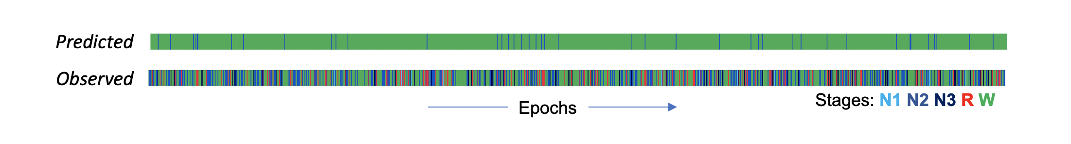
Confusion matrix: 5-level classification: kappa = 0.02, acc = 0.52, MCC = 0.05
If we look at the stages observed (bottom row, one line is one epoch) versus the SOAP-based predictions (top row), we see there is little correspondence. In fact, most epochs have been predicted to be wake. The precise predictions aren't of particular interest here, in the context of a very low overall kappa - it simply means that the model was not able to find stage-relevant information in the EEG (i.e. precisely because we scrambled it).
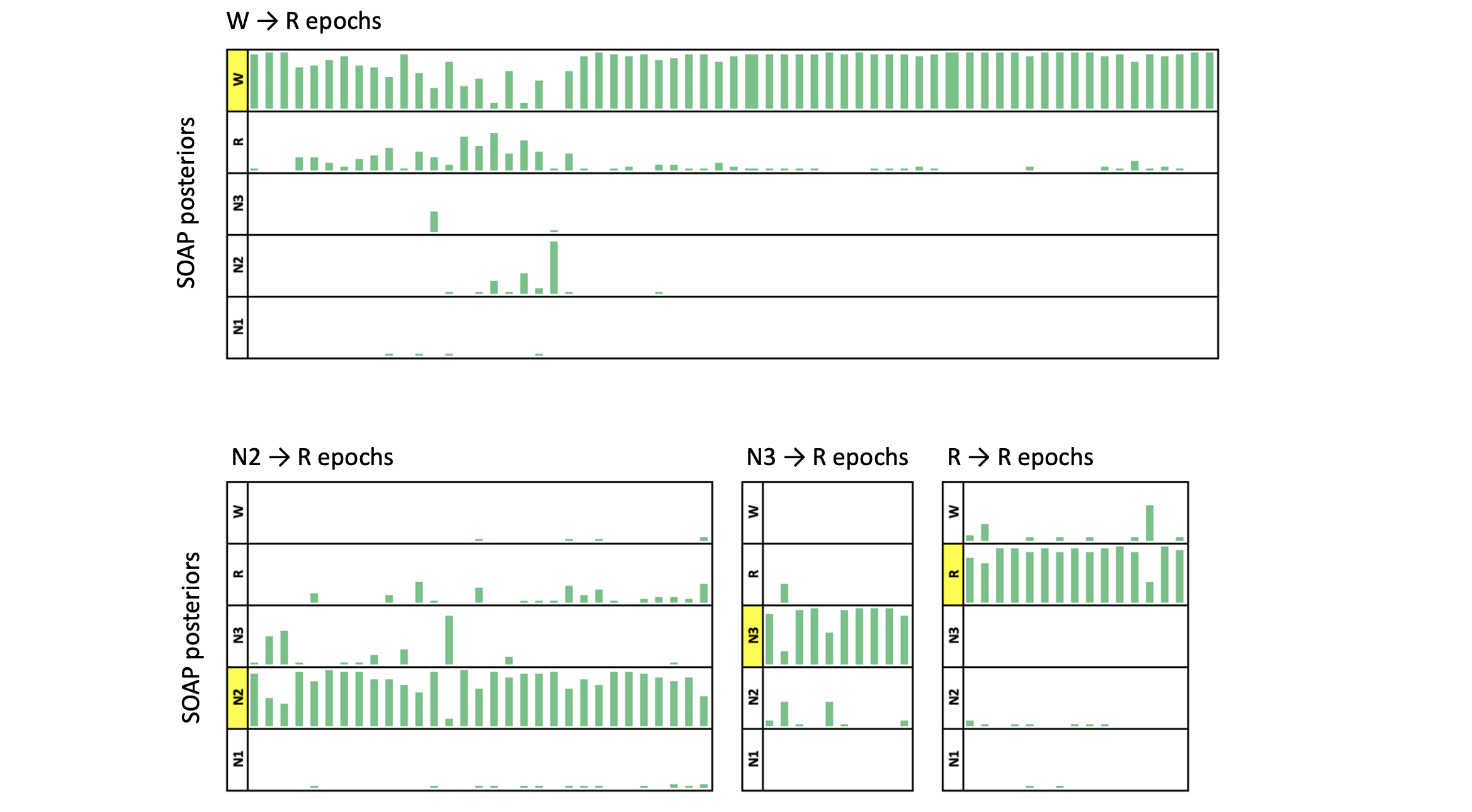
We can also look at the posterior probabilities as well as the most-likely stages under the SOAP model. (The POPS output follows the same structure.) Here we see the posteriors from the original SOAP analysis (i.e. with the true/observed staging). Each line shows the probabilities "stacked" to sum to 1.0, for a given epoch. In the real data, the predictions were "confident" in the sense that the maximum posterior was typically near 1.0. In contrast, the completely scrambled data shows a very different pattern (note, the plots are sorted such that the most likely stage is plotted at the bottom):
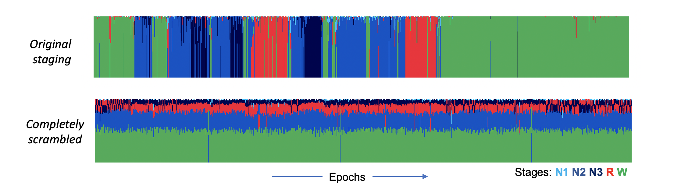
If you ever see this type of pattern (plus a low kappa), it is telling you there is little or no correspondence between signals and stages.
Hint
In this (contrived) example, depending on the randomization
of stages, it is possible that you don't even have a single SVD
component that is associated with the stage data, in which case
the LDA/QDA model will not be fit. If this were to occur, you can
make the inclusion of components more liberal by setting pc to a
higher value, e.g. 0.2
luna a.lst -o soap0.db annot-file=rnd.eannot -s SOAP epoch pc=0.2
retaining 4 of 10 PSCs, based on ANOVA p<0.2
Swapped files
In the previous example, any quick visual inspection of the observed
hypnogram (i.e. corresponding to the Observed stages plot above) would
indicate that the data are not consistent with a typical looking human
hypnogram, and so we wouldn't really need SOAP to tell us that. What
if we did have stages that looked sensible, but did not align with
the individual on whom we have signal data though? To see, here we
swap another person's staging in, and see what happens. i.e. here the stages in other.eannot
are from somebody else:
luna a.lst -o soap2.db annot-file=other.eannot -s SOAP epoch
Confusion matrix: 5-level classification: kappa = 0.29, acc = 0.55, MCC = 0.32
This certainly reflects some degree of over-fitting, whereby the LDA is trying hard to find connections between the signals and stages. This level of value is still a lot lower than what we'd expect normally, however. Here are the two hypnograms:
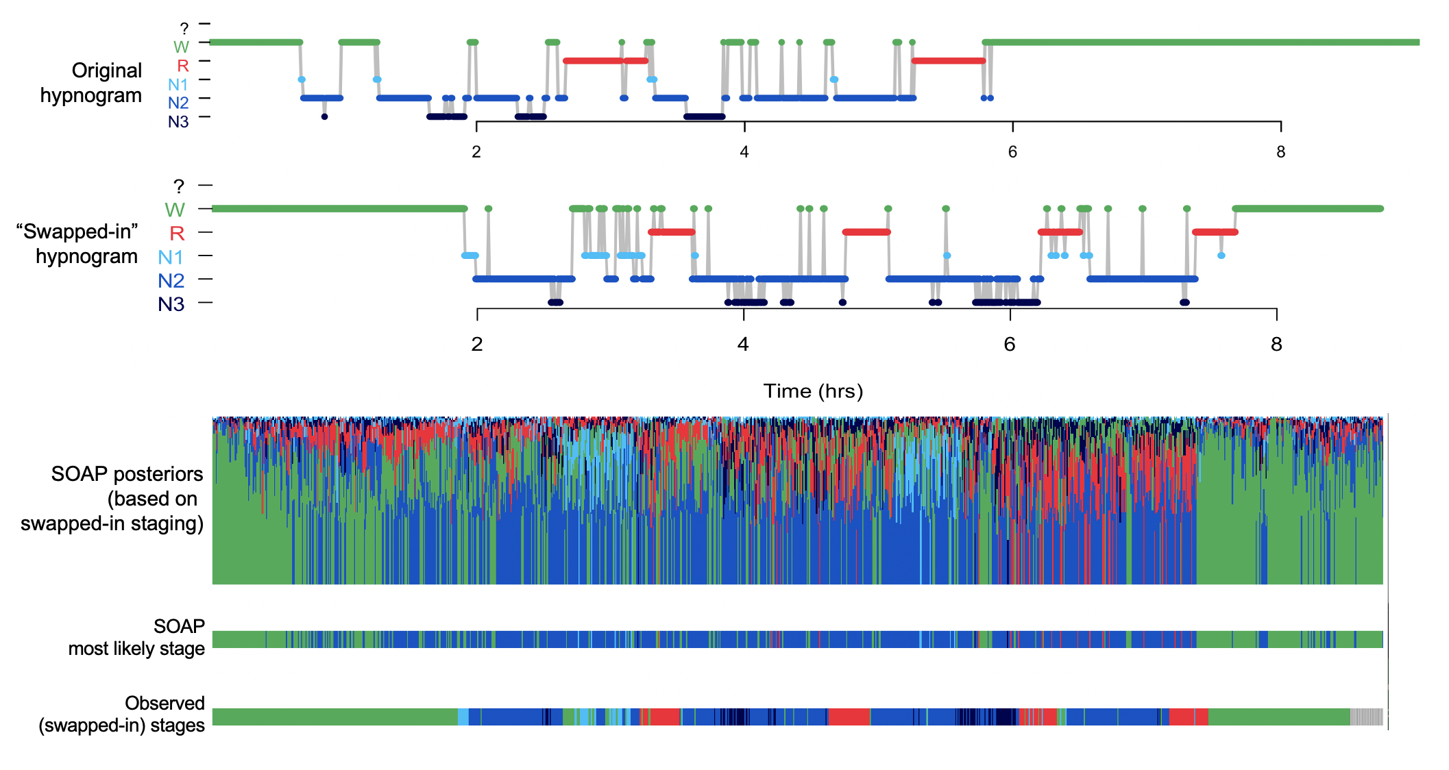
They are clearly different, but still, they are more similar than the completely random set. For example, both studies start and end in quite long periods of wake. This enables the model to achieve an above-chance level of wake/sleep classification, perhaps, but again it is nowhere near the level of performance we'd expect with real data:
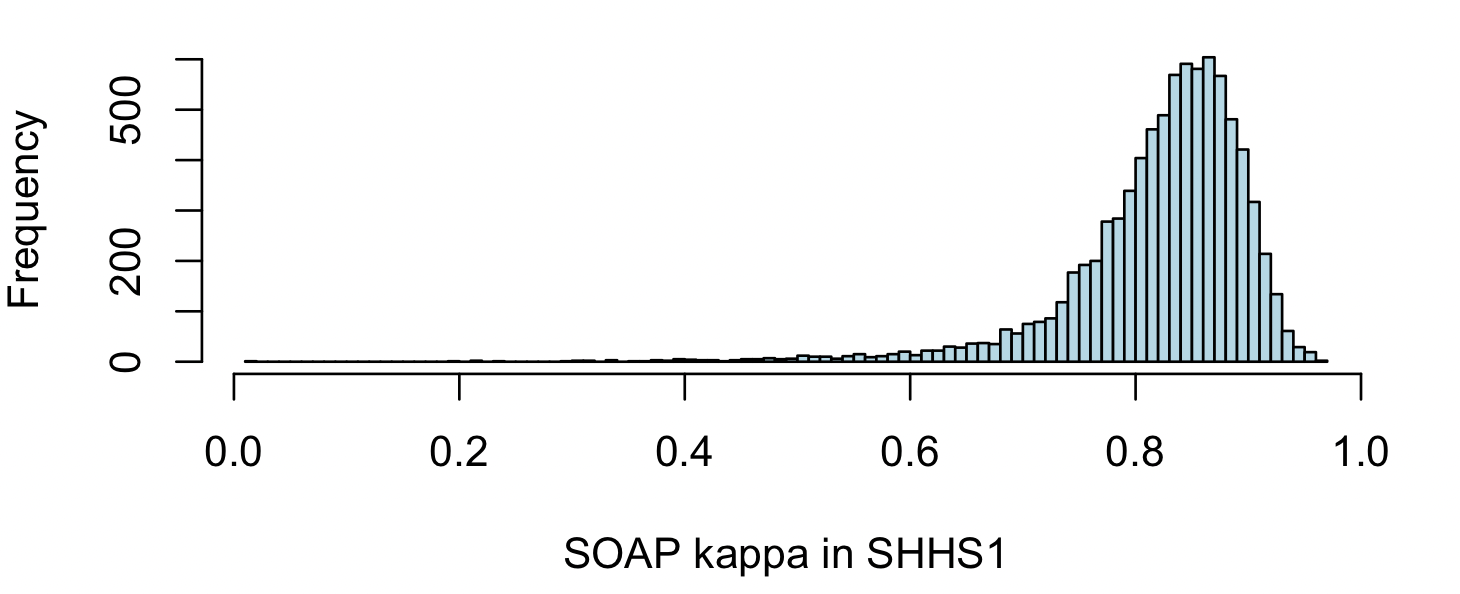
To contextualize this result, here is a histogram of kappa values from thousands of people in the SHHS (wave 1) -- values of kappa under 0.5 are very rare, and likely indicate (major) issues with the staging. Most individuals have kappas of 0.8 or greater:
Remember that because SOAP fits and predicts on the same data, this kappa should not be interpreted in the same way as a kappa from a true prediction context. This just means the absolute values are calibrated differently. Nonetheless, it still is informative as to the quality of staging, as we show below.
Stage completion
In some circumstances, SOAP can be used to "fill in" missing data from
a partially scored study ( (as long as a sufficient number of epochs
have been scored for each stage). For example, going back to the original staging, let's pretend
that we only staged the first 600 epochs, here making a new file inc.eannot that is incomplete, placing
? symbols for all epochs past 600:
awk ' NR <= 600 { print $0 } NR > 600 { print "?" } ' obs.eannot > inc.eannot
luna a.lst -o soap3.db annot-file=inc.eannot -s SOAP epoch
Confusion matrix: 5-level classification: kappa = 0.87, acc = 0.92, MCC = 0.88
Confusion matrix: 3-level classification: kappa = 0.92, acc = 0.96, MCC = 0.92
final epoch counts: ?:484 N1:10 N2:275 N3:84 R:68 W:163
# full original
k <- ldb( "soap1.db" )

# completed (missing after epoch 600)
m <- ldb( "soap3.db" )

par(mfcol=c(3,1) , mar=c(1,3,0.5,0.5) )
lhypno( k$SOAP$E$PRIOR )
lhypno( m$SOAP$E$PRIOR )
lhypno( m$SOAP$E$PRED )
Error correction
On the assumption that most epochs have been correctly and consistently assigned, we may expect a high kappa value from SOAP. Under this scenario, we can then use SOAP in a different manner, to potentially identify and correct a smaller number of inconsistencies or errors in staging that may exist.
On the assumption of largely correct staging, SOAP confidence scores/kappas can also provide a rough guide to signal quality. For example, given multiple EEG channels, if some have very high kappas but some have low kappas, the latter set may contain higher levels of artifact, etc.
SOAP also generate probabilistic stage assignments based on the original categorical/discrete staging. This may be useful, for example, to restrict certain analyses only to "high confidence" intervals, or to derive hypnogram statistics (e.g. stage duration) based on probabilistically-weighted epoch counts. Although beyond the scope of this vignette, this approach may better handle "mixed epochs", if the SOAP model places weight on multiple stages.
That is, overall SOAP can be viewed in two ways: 1) as a tool to check the consistency between signals & staging, 2) as a tool to manipulate/use the existing staging, on the assumption that stages and signals are largely consistent.
Here we consider a biased/inconsistent stager, who (for some strange reason) scores every ninth epoch as REM. We can simulate that as follows:
awk ' NR % 9 != 0 { print $0 } NR % 9 == 0 { print "R" } ' obs.eannot > err.eannot
err.eannot:
luna a.lst -o soap4.db annot-file=err.eannot -s SOAP epoch
Confusion matrix: 5-level classification: kappa = 0.74, acc = 0.83, MCC = 0.75
In this particular case, given a reasonably high kappa, we might do well to accept these revised predictions over the original ones. That is, when SOAP changes the staging for an epoch, it is really saying (for example): "although staged R, this epoch looks much more like most of the other epochs labelled N3, than it does to most of the other epochs labelled R". Naturally there is no guarantee that any changes SOAP makes will always be the correct ones. In some cases, it might be more likely to make staging worse on average, not better -- this will in large part depend on the (unknowable) type of data, and the types/extent of staging errors made. In future work, we plan to evaluate empirically the conditions under which using SOAP may improve staging quality, e.g. using correlations between known demographic factors such as age, or test-retest reliability, as figures of merit (assuming that more reliable staging will increase the strength of statistical associations).
Hint
New/revised SOAP stages can be obtained from the PRED column of the E-stratified output tables.
Aligning orphaned stage data
The PLACE command implements a special case of using SOAP to align
staging with signal data. Specifically, this addresses the scenario
where an EDF and a set of annotations differ in length, but one is not
sure how they should be aligned (i.e. does the list of annotations
necessarily start at the 0-second EDF start, or some other time)?
Although this may be considered a niche case, we have come across
exactly this type of scenario more than once when working with legacy
datasets - e.g. as might happen if only parts of the night were
extracted for much longer / 24-hour recordings, and the time-stamps
have been lost during the export process, with original datasets no
longer available. (If nothing else, it is a nice proof-of-principle demonstration of the SOAP model.)
We'll again simulate this type of scenario, here extracting out only staging data from epoch 30 to 730 (i.e. 601 epochs, whereas the full EDF/staging has 1084 epochs).
awk ' NR >= 30 && NR <= 730 ' obs.eannot > ex.eannot
The PLACE command is essentially a wrapper around SOAP, which
calls it multiple times, at all possible alignments of the staging and
signal data. (The staging may be shorter, or longer, than the EDF
signals.) Graphically, this illustrates what PLACE is doing:
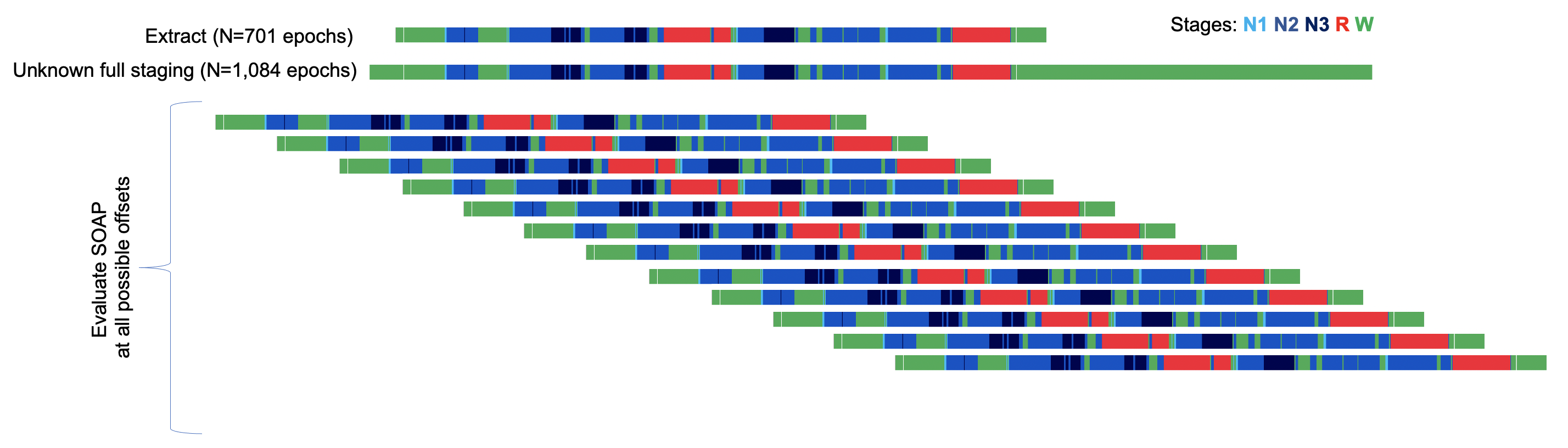
For every placement, it calculates the SOAP kappa, and then will, at the end, select the offset with the highest kappa as the most likely placement.
We run PLACE as follows:
luna a.lst -o place.db -s PLACE stages=ex.eannot
stages command, and some other specific options, this command takes the same options as the SOAP command (i.e.
this will assume a single-EEG model for C4_M1 by default.
destrat place.db +PLACE | behead
             K   0.86073512269087
        OFFSET   29
      OLAP_EDF   0.646678966789668
        OLAP_N   701
      OLAP_STG   1
Here we see the most likely offset is 29, which is the correct
answer (i.e. staging epoch 1 corresponds signal epoch 1+29 = 30,
based on how we extracted the epochs above). We can plot the kappa for
all possible alignments, to get a sense of how specific this placement was:
destrat place.db +PLACE -r OFFSET > o.1
d <- read.table("o.1",header=T,stringsAsFactor=F)
plot( d$OFFSET , d$K , type="n" , xlab="Offset (epochs)" , ylab="Kappa" )
abline(v=c(0,29), col=c("gray","red") )
lines( d$OFFSET , d$K , type="l" ,  col="darkgreen" )
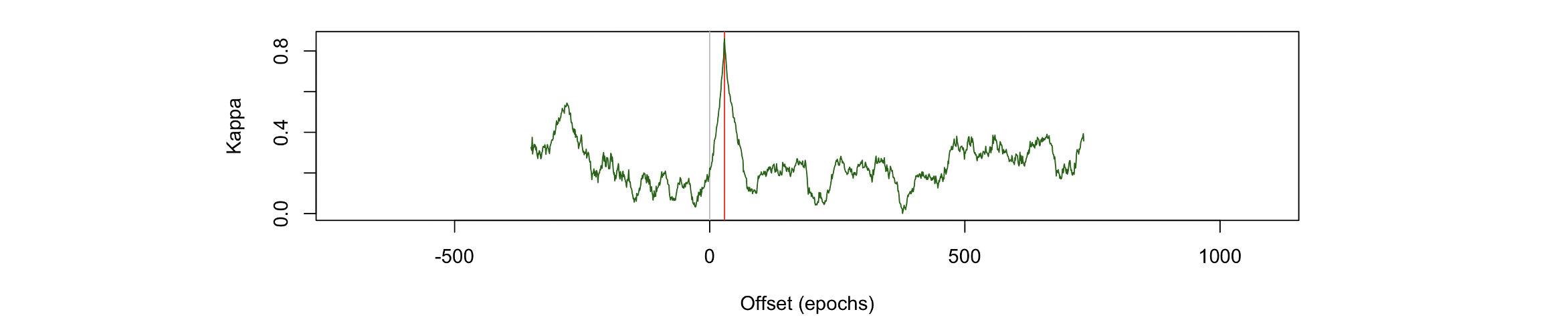
We see there really is quite a marked spike at the exact true offset.
Although it will depend on a number of factors, and there are
certainly scenarios that could mislead PLACE, in general, with
reasonably typical inputs, the PLACE command appears to do a good
job of resolving alignments within a single epoch.
Of course, one might say: why not just use an automated stager,
rather than trying to rescue partial, manual staging? This is also a
reasonable idea - we could do so with POPS below, for example.
However, there may be circumstances where the montages are very
different (e.g. only intracranial EEG leads, or from a wearable
device, or a non-human model system for which good staging models have
not been built). If one is other confident in the quality of the
human staging, it still may be preferrable to automated staging, and
given it has already been performed, it makes sense to try to use it
if you can.
Changing epoch durations
The SOAP model is not constrained to 30-second epochs. In fact, you can easily change the epoch size to obtain any desired epoch length: e.g. for 10-second epochs
luna s.lst -o out.db -s 'EPOCH dur=10 & SOAP epoch '
This will emit 3,252 stage predictions, rather than 1,084 (from the 30-second epoch). However, in practice, one wants to ensure that the original epoch durations are an exact multiple of any smaller epoch time used: if not (e.g. specifying a 7-second epoch, but with original 30-second staging), then some epochs may have more than one assigned stage.
However, with the REBASE variant of the SOAP command, it is also
possible to fit a model based on epoch features of one particular
duration, but then to make predictions at a second duration. Thus enables
one to, for example, translate between 30-second and 20-second epoch durations,
or vice versa. The key is that a third epoch length must be selected so that
both are exact multiples: e.g. 10 or 5 seconds.
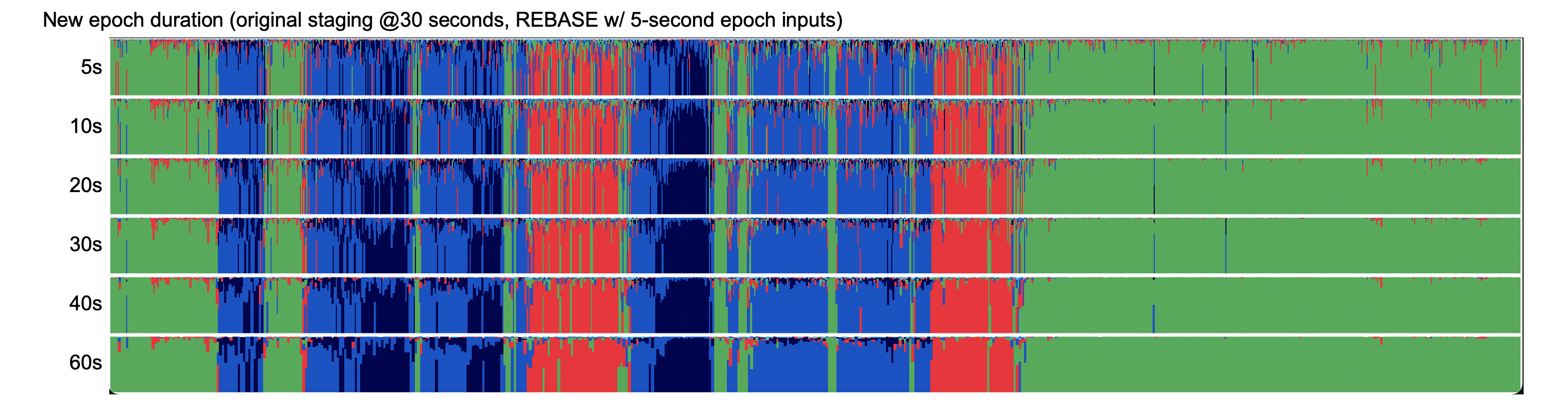
For example, given original 30-second staging, this builds a SOAP model of the signal-stage relationships based on 5-second sub-epochs, but then uses that to predict given features based on 20-epochs of the same data:
luna s.lst -o out.db -s 'EPOCH dur=5 & REBASE dur=20'
This command may have some utility if working with studies based on
European/US 20/30-second staging conventions, but you wish to
harmonize them. As noted above, simply running automated staging with the desired epoch
duration is also an option, e.g. using POPS.
Here we see posterior probability plots for a range of rebased epoch durations:
Prediction with POPS
Finally, instead of seeding analysis on observed staging, we can
predict stages from scratch, given a model based on other PSGs.
This is what the POPS command does.
LGBM & POPS development
POPS implements feature-based prediction using Microsoft's LightGBM gradient descent boosting machine library. The POPS command is conceptually similar to Raphael Vallat's excellent YASA Python-based stager, which also uses LightGBM although with slightly different feature sets. (FWIW, in work to be described more fully, we've found average performance to be broadly comparable between POPS and YASA - although perhaps interestingly, the kappas from the two models are often not very strongly correlated, suggesting there may be room for improvement, i.e. if the two implementations tend to have different failure modes...
Single-channel EEG model
Fully detailing this model, its variations, and the procedure for
training models is beyond the scope of this vignette. Here, we merely
show performance for this one SHHS individual, using a beta-version
of the vanilla single-EEG model. The only requirement is a central
EEG (or equivalent) channel labelled C4_M1 (you can use the alias
options as noted above).
This library (m1) is available for download at this Dropbox
link. This is
a ZIP file (13MB) called m1.zip. After downloading, expanding it will
result in a folder called m1 (model 1). You then will run POPS
using lib to specify the model root (m1) and path to point to
this folder (e.g. ~/working/sleep/pops/m1 or wherever you saved it).
The m1.ftr file defines the set of features extracted per epoch,
upon which the model is trained. Naturally, this is also necessary
when using the model for prediction, as Luna needs to be able to
derive the same set of features in new data. The details aren't
important here, but this is the current prototype version of the
default single-EEG model:
% --------------------------------------------------------------------------------
%
% Declare any channels used (required), sample rates
%
% --------------------------------------------------------------------------------

CH C4_M1 C4 C4.M1 C4-M1 C4.A1 C4_A1 C4-A1 128 uV

% --------------------------------------------------------------------------------
%
% Level 1 features
%  block : feature {key=value key=value}
%
% --------------------------------------------------------------------------------

% full power spectra, up to 30 Hz
spec1:  SPEC  C4_M1  lwr=0.5 upr=30
vspec1: VSPEC C4_M1  lwr=0.5 upr=30

% bands (relative band power)
rband1: RBAND C4_M1

% alternate metrics

misc1: HJORTH   C4_M1
misc1: SKEW     C4_M1
misc1: KURTOSIS C4_M1

misc2: FD       C4_M1
misc2: PE from=5 to=5  C4_M1

% indiv-level covariates, if available

demo1: COVAR age male

% --------------------------------------------------------------------------------
%
% Epoch/row exclusions based on level-1 features
%
% --------------------------------------------------------------------------------

misc1: OUTLIERS th=8

% --------------------------------------------------------------------------------
%
% Level 2 features:
%  to-block: feature block=from-block {key=value}
%
% --------------------------------------------------------------------------------

% SVD - in trainer model, writes this to myfile.txt (based on all individuals)

spec1.svd:  SVD block=spec1 nc=8 file=m1.spec1.svd
vspec1.svd: SVD block=vspec1 nc=4 file=m1.vspec1.svd

% temporal smoothing
spec1.svd.smoothed: SMOOTH block=spec1.svd half-window=15
spec1.svd.denoised: DENOISE block=spec1.svd lambda=0.5

rband1.smoothed: SMOOTH block=rband1 half-window=15
rband1.denoised: DENOISE block=rband1 lambda=0.5

misc1.smoothed: SMOOTH block=misc1 half-window=15
misc1.denoised: DENOISE block=misc1 lambda=0.5

misc2.smoothed: SMOOTH block=misc2 half-window=15
misc2.denoised: DENOISE block=misc2 lambda=0.5

time1: TIME order=1

rband.deriv: DERIV block=rband1 half-window=20
spec1.svd.smoothed.deriv: DERIV block=spec1.svd.smoothed half-window=20


% --------------------------------------------------------------------------------
%
% Final feature selection (blocks as defined above)
%
% --------------------------------------------------------------------------------

SELECT demo1 rband1 misc1 misc2 spec1.svd vspec1.svd
   spec1.svd.smoothed spec1.svd.denoised rband1.smoothed rband1.denoised
   misc1.smoothed misc1.denoised misc2.smoothed misc2.denoised time1
   rband.deriv spec1.svd.smoothed.deriv
Running POPS
To run POPS, just invoke:
luna s.lst -o pops.db -s POPS path=~/dropbox/pops/m1 lib=m1
path points to where you downloaded the m1 folder (see above).
This should finish quickly - it typically takes around 2 seconds to fully stage a study. If the signal is of a different sample rate, Luna will first resample to obtain a 128 Hz signal.
POPS and LGBM support
If you try to run POPS or similar commands and see the following:
error : no LGBM support compiled in
If manual staging was available, Luna will calculate kappa statistics and a confusion matrix. (Note: unlike SOAP, any original staging information is not used in any of the calculations/predictions; it is only included to evaluate model performance, when the "true" answers are known):
  kappa = 0.897767; 3-class kappa = 0.940477 (n = 1082 epochs)

Confusion matrix:
        Pred:    W       R       N1       N2       N3        Tot
  Obs: W       528       0       14       14        0       0.51
       R         4     124       0         2        0       0.12
       N1        0       0       1         9        0       0.01
       N2        1       3       1       290        7       0.28
       N3        0       0       0        16       68       0.08
       Tot:   0.49    0.12    0.01      0.31     0.07       1.00
Here we see a very high of almost 0.9 for the 5-class solution. Correspondingly, the confusion matrix shows very little evidence of much confusion in these stage assignments.
Human-human inter-rater reliability in staging is typically only around kappa ~0.8, so these types of results definitely reflect an upper-bound on how good we'd expect a stager to be. We're in the process of evaluating, but in general POPS has good performance, with a typical kappa of around 0.8 for the 5-class problem, and higher for the 3-class problem. The exact parameters of performance will of course always depend on a host of factors - especially when applied to studies from completely different cohorts than used in the training of the model. (This particular SHHS individual was not used in model training, although other SHHS individuals were.) For future development, we are most focused on making the predictions more robust (in the sense of trying to avoid doing very poorly, even when in principle the signal data are sufficient), rather than trying to add one or two percentage points to the (already high) average kappa values. A full description of the approach - and various extensions to it under development - will be detailed in future updates.
The key metrics are available in the output databases (some rows omitted for clarity):
destrat pops.db +POPS | behead
             ACC   0.934380776340111
            ACC3   0.964879852125693
            CONF   0.892255280246547
               K   0.897767498309929
              K3   0.940476638571775
             MCC   0.898677254612086
            MCC3   0.941308923450242
     REM_LAT_OBS   118.5
     REM_LAT_PRD   124
     SLP_LAT_OBS   41
     SLP_LAT_PRD   36.5
The confusion matrix from the console can also be extracted (although note the wonky row/col ordering here):
destrat pops.db +POPS -r OBS -c PRED -v N
ID            OBS    N.PRED_N1  N.PRED_N2  N.PRED_N3  N.PRED_R   N.PRED_W
shhs1-0000    W      14         14         0          0          528
shhs1-0000    R      0          2          0          124        4
shhs1-0000    N1     1          9          0          0          0
shhs1-0000    N2     1          290        7          3          1
shhs1-0000    N3     0          16         68         0          0
Summary statistics such as stage durations based either one counts of the most likely epoch (PR1) or a weighted estimate
(PRF) can be obtained under the SS stratum:
destrat pops.db +POPS -r SS -p 3
ID            SS      F1      OBS     ORIG    PR1     PREC    PRF     RECALL
shhs1-0000    W       0.970   278.000 278.500 266.500 0.991   255.314 0.950
shhs1-0000    R       0.965   65.000  65.000  63.500  0.976   61.512  0.954
shhs1-0000    N1      0.077   5.000   5.000   8.000   0.062   27.338  0.100
shhs1-0000    N2      0.916   151.000 151.500 165.500 0.876   161.227 0.960
shhs1-0000    N3      0.855   42.000  42.000  37.500  0.907   35.610  0.810
shhs1-0000    ?       NA      1.000   0.000   1.000   NA      1.000   NA
Finally, the raw epoch-level predictions can be obtained as follows (PRED):
destrat pops.db +POPS -r E -p 3
ID            E  CONF    FLAG    PP_N1   PP_N2   PP_N3   PP_R    PP_W    PRED    PRIOR
shhs1-0000    1  0.998   0.000   0.002   0.001   0.000   0.000   0.998   W       W
shhs1-0000    2  0.996   0.000   0.003   0.001   0.000   0.000   0.996   W       W
shhs1-0000    3  0.999   0.000   0.001   0.001   0.000   0.000   0.999   W       W
shhs1-0000    4  0.997   0.000   0.002   0.000   0.000   0.000   0.997   W       W
shhs1-0000    5  0.998   0.000   0.002   0.000   0.000   0.000   0.998   W       W
shhs1-0000    6  0.996   0.000   0.002   0.002   0.000   0.000   0.996   W       W
shhs1-0000    7  0.997   0.000   0.001   0.001   0.000   0.000   0.997   W       W
shhs1-0000    8  0.997   0.000   0.002   0.001   0.000   0.000   0.997   W       W
shhs1-0000    9  0.996   0.000   0.002   0.002   0.000   0.000   0.996   W       W
...
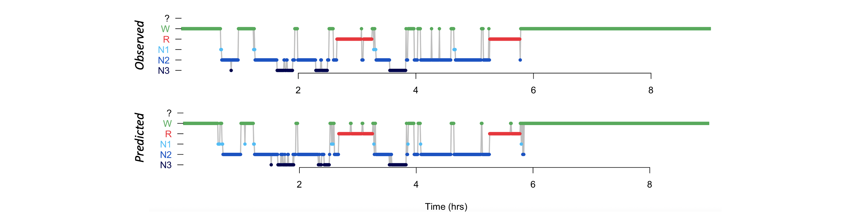
Using lunaR, we can plot the observed and POPS-predicted hypnograms:
k <- ldb("pops.db")
> par(mfrow=c(2,1))
> lhypno( k$POPS$E$PRIOR )
> lhypno( k$POPS$E$PRED )
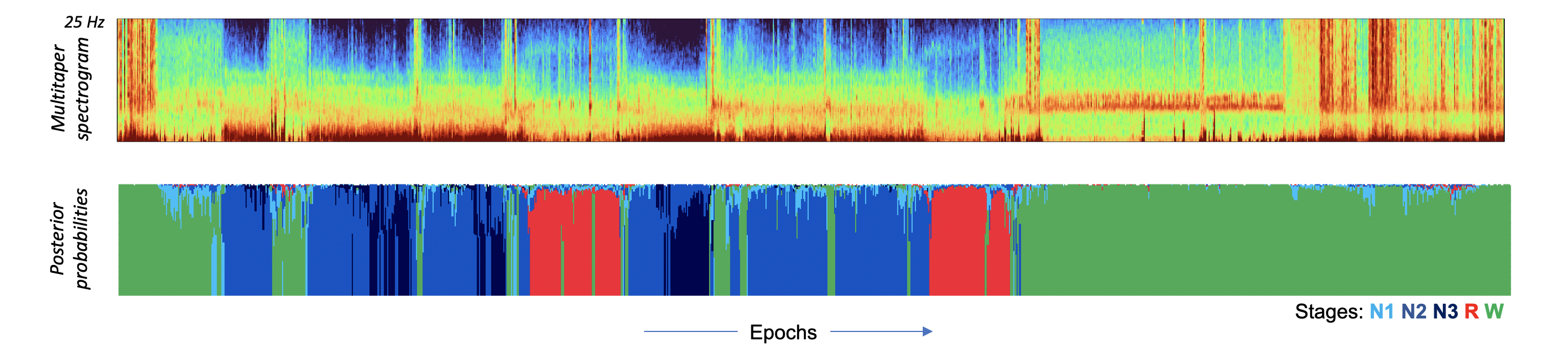
We can also plot the posterior probabilities, in the same way we did for SOAP. Here we'll also output the multi-taper spectrogram for visual reference: i.e. we separately extracted that here:
luna a.lst -t mtm -s MTM sig=C4_M1 nw=15 epoch
d <- read.table( "mtm/shhs1-0000/MTM_F_CH_SEG.txt.gz" , header=T, stringsAsFactors=F )
Conclusion
This was an introduction to some of the logic and potential applications of the SOAP (stage evaluation) command, as well as a quick skim of the POPS command for staging, currently in the context of a single-channel EEG. We'll be posting updates to the model syntax, options and newly trained models in the near future... Stay tuned!