Moonlight
Overview
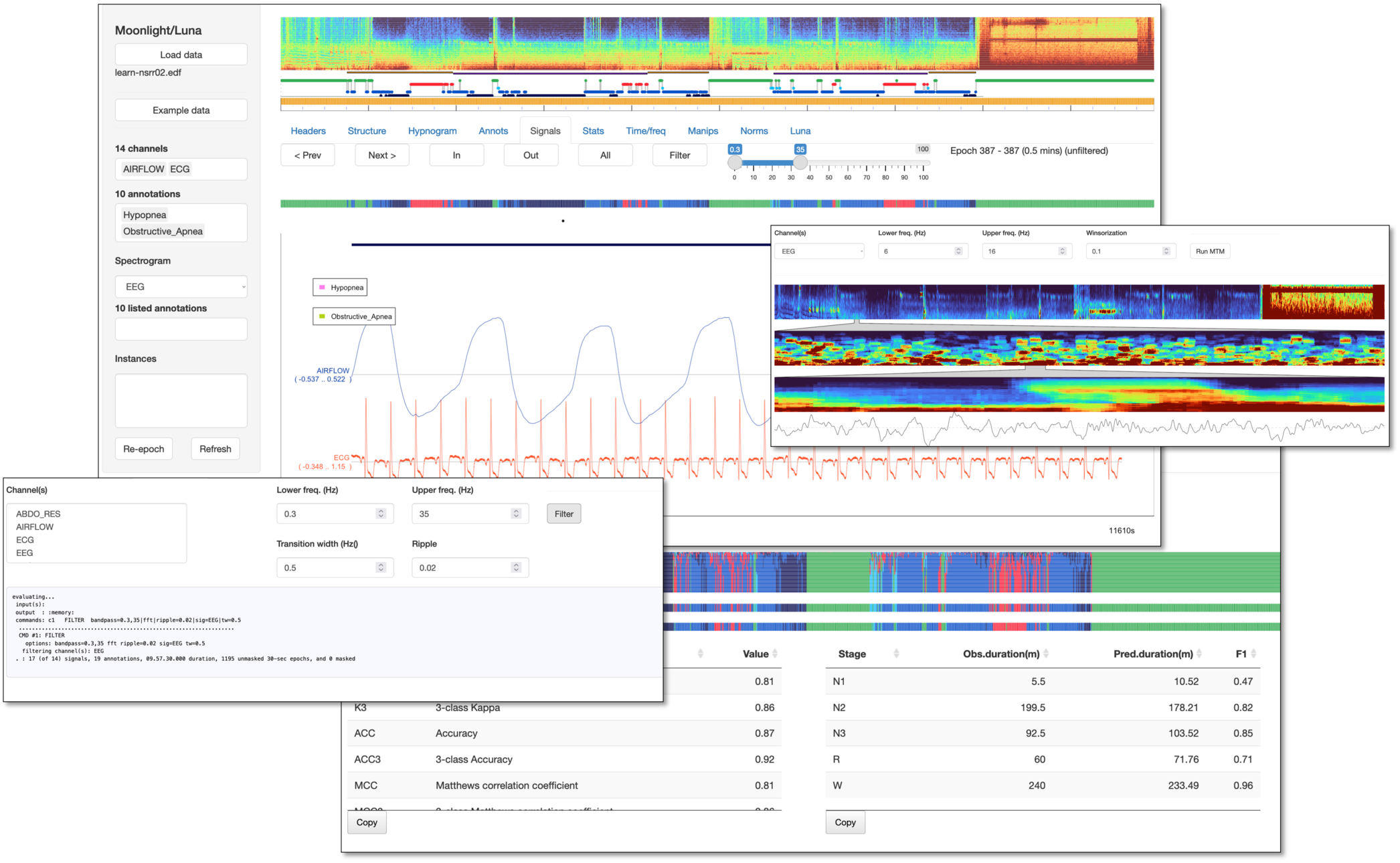
Moonlight is a Luna-based interactive viewer for EDF signal and annotation data, specifically designed for polysomnographic data. As well as visualization, Moonlight supports basic analyses and manipulation of sleep data, a range of summary statistics, and hypnogram-based analyses including automated staging using POPS. Below we give a brief tour of the current main components.
Moonbeam & National Sleep Research Resource Data
Moonlight also includes the Moonbeam extension that allows NSRR users to directly pull NSRR signal data into Moonlight via the web, described here
Moonlight development and scope
Moonlight is actively under development - please let us know of any rough edges or missing functionality. Note that Moonlight is not designed to be a performant, general purpose EDF viewer, although it does support basic viewing abilities. The niche Moonlight attempts to fill is to provide some sleep-specific functionality (including hypnogram statistics and automated staging) as well as tight coupling of Luna analyses, i.e. the ability to actively manipulate PSG data in this context. It also provides tools for viewing annotation data alongside signal data.
Access
See these notes on how to access Moonlight. Briefly, you can:
-
use our AWS hosted instances at http://remnrem.net/. Advantages: no installation. Disadvantages: slower to upload EDFs to the cloud, limited number of instances available at any one time
-
pull our Dockerized version of luna and run from there. Advantages: runs on all platforms that can support Docker Desktop (see here). Disadvantages: requires Docker set up; some Docker versions can currently have slow I/O under default configurations on certain platforms
-
run directly from a local version of lunaR: Advantages: most flexible and fastest option. Disadvantages: requires installation of R and lunaR
Basic principles
Moonlight is designed to upload a single EDF (or EDF+) at a time, optionally along with one or more annotation files. You can then view basic properties of the data, including viewing raw signals. The window contains a number of panels, all of which show some aspect of the uploaded EDF:
-
Left panel : select files to upload and which channels/annotations to view
-
Headers : basic EDF headers
-
Structure : epoch level structure of the data, showing discontinuities (from masking or EDF+D)
-
Hypnogram : hypnogram-based summaries as well as automated staging (POPS) and stage evaluation (SOAP)
-
Annots : visualization and tabulation of annotations
-
Signals : raw signal viewer (including annotations)
-
Stats : basic signal summary statistics (e.g. means, skewness, etc)
-
Time/freq : several whole-night representations: multi-taper spectrograms, Hjorth-plots, and epoch-level time-series clustering
-
Manips : manipulations of the attached signals: resampling, rereferencing, filtering, copying, renaming, etc
-
Models : prototypes of predictive models and population-based norms model for EEG and other metrics
-
Luna : evaluation of arbitrary Luna commands
The easiest way to learn is to open an instance at http://remnrem.net/ and load the Example data (one of the NSRR tutorial individuals from the SHHS) and/or follow this tutorial which uses Moonlight to step through the the Luna and lunaR tutorial pages.
Left panel
Load data
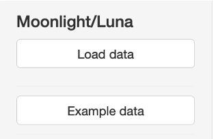
To attach an EDF (and optionally annotation files) select Load data from the top of the left panel. Note that depending how Moonlight is configured (e.g. running locally versus on the web), the load button/dialog box may look slightly different (either left or right boxes):
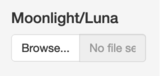
With either dialog box, you can upload:
-
a single EDF or EDF+ files (which must end in the extension
.edf). If multiple EDFs are selected, only the first will be uploaded. -
annotation files in Luna .annot format, Luna .eannot or NSRR-style XML formats (ending either
.annot,.eannotor.xml). If multiple files are selected, all will be uploaded (and assumed to match the uploaded EDF). -
All files need to be uploaded at the same time: this means that currently, all files must be in the same folder, in order that they can be concurrently selected.
Example data
Instead of uploading your own data, to try out Moonlight you can
alternatively click Example data to attach the NSRR tutorial
(learn-nsrr02) file along with the associated XML annotation file:
Channels
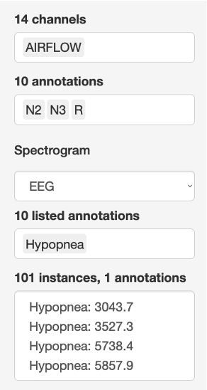
After uploading, the EDF channels will be available in the list box Channels. Multiple channels can be selected. Selected channels indicate those that will be shown in the Signals tab, and for cetain other panels (e.g. Stats). Note that some panels have their own channel selection method (e.g. the Manips panel, or the multi-taper spectrogram panel), and so they ignore this box. When signals are added to (or removed from) the dataset, this list will be updated.
The image below shows the Channels list box, along with other widgets described below.
Annotations
As above, this list mirrors the Channels list, and determines which annotations are shown in the Annots and Signals panels. Multiple annotations can be selected.
Spectrogram
This list selects a single channel (typically an EEG) to be used to generate the Spectrogram at the top of the main window. Note one wrinkle: this doesn't automatically update after masking/restructuring a dataset (deleting epochs). To update it, one currently must select a second channel, then go back to the first.
Listed annotations
Whereas the top Annotations list indicates which annotations will be shown, this second box determines which annotation events are listed in the Instances box below.
Instances
If Listed Annotations are selected, any events will be listed in this box. Clicking on an entry when viewing the Signals panel will move the window to the epoch(s) containing that event. For events less than 10 seconds in duration, a single 30-second window is selected. For longer events, multiple epochs will be shown, centered around the selected event.
Re-epoch
After masking epochs (e.g. via the Manips/Mask panel, or directly
running MASK via the Luna panel), this button will effectively run
a RESTRUCTURE command, to actually remove those masked epochs from
the (in-memory) dataset.
Refresh
Clicking Refresh returns the in-memory dataset to as it was when the files were first uploaded. i.e. any masks, new channels and other changes are dropped. It should be the same as reloading a file (but will be quicker).
Spectrogram/hypnogram
Based on the channel selected in the Spectrogam list (left panel),
Moonlight generates a spectrogram using Welch's method and Luna's
PSD command. The x-axis is all currently included epochs; the
y-axis is 0.5 to 25 Hz; the z-axis (color) is the log-scaled spectral
power. Note that only signals with a sample rate of 50 Hz or more are
included in the Spectrogram list.
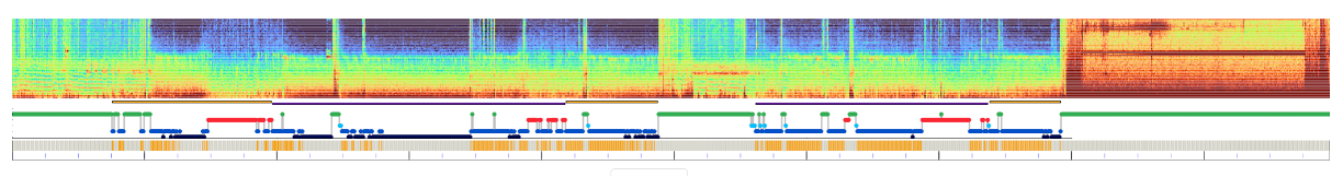
Below the spectrogram, if sleep stage are available, Luna will output a hypnogram (red=REM, green=wake, yellow=Lights, gray=unknown, light-dark blue=N1, N2 and N3) in 30-second epochs. NREM cycles are estimated and shown as alternating orange/purple bars above the hypnogram.
You can select a range by clicking and dragging on the hypnogram to
define the Lights Out range - all epochs before and after will be
set to L internally - these changes will be respected by the POPS
stager - i.e. only epochs within the Lights Out interval will be
staged.
Finally, Below the hypnogram, a small bar plot shows which epochs are
currently masked (gray) or not (orange). Running Re-epoch (or
RESTRUCTURE) will remove gray epochs (and plot them as white,
i.e. gaps) in this plot. If a dataset has been masked and re-epoched in this way, the
spectrogram will only show included epochs:
In contrast, (unless different Lights Off/on markers are set) the hypnogram is only calculated once, when first uploading the data and based on all epochs.
Headers

The first panel in the main window gives a simple tabulation of the main EDF header values: overall (left) and per channel (right).
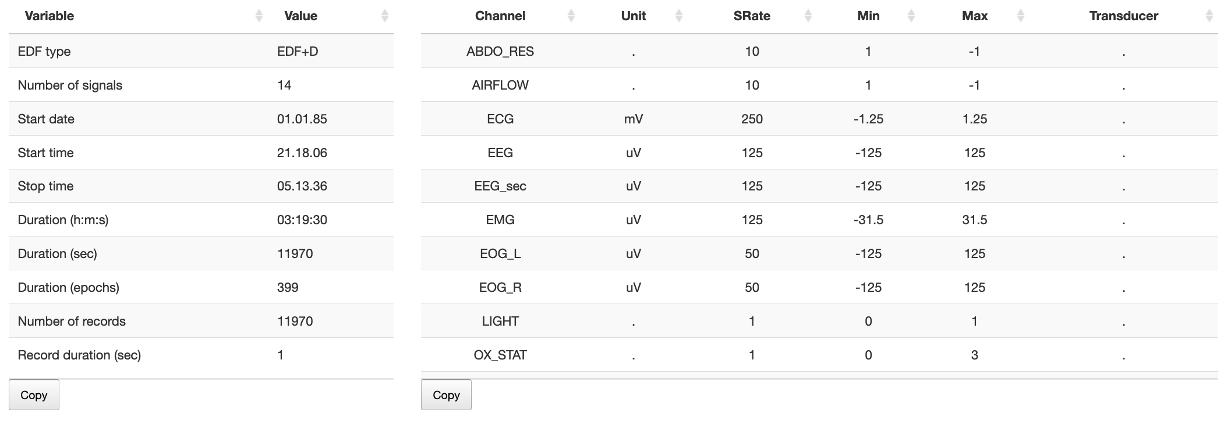
Note that the tables are scrollable (e.g. if the number of rows is too great to display) and can be copied to the Clipboard by clicking the Copy button.
Structure
This panel shows the epoch-level structure of a dataset.
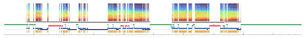
Segments
This panel is only useful for EDF+D files (i.e. those with
discontinuities, i.e. gaps. Internally, this runs Luna's
SEGMENTS command and graphs the output. If epochs have subsequently
been dropped (from either an EDF/EDF+C or EDF+D) then the lower
figures show these selected epochs - i.e. what constitutes the current
in-memory dataset, which may contain gaps, e.g. after selecting only
N2 epochs.
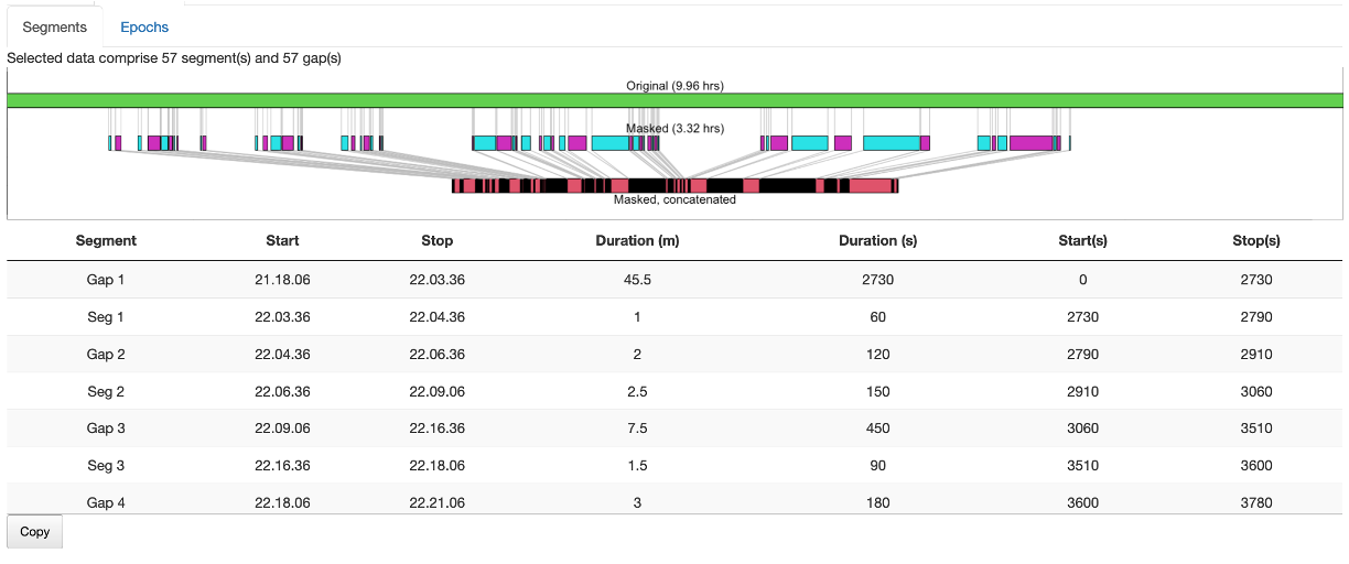
The table below the plot shows actual times of segments/gaps in the data.
Epochs
This panel shows three tables of the epochs in the dataset (30-seconds): 1) for the initial dataset, aligned to the EDF start, 2) for the initial dataset, aligned to sleep staging, 3) for the current in-memory dataset, aligned to staging annotations. See the tutorial for an example.
Hypnogram
As well as generating the hypnogram in the top of the display, Moonlight derives numerous statistics based on the hypnogram, shown in various sub-panels as described below. All metrics are based on the staging uploaded at the study start (i.e. rather than SOAP/POPS staging).
Summaries
Basic summaries from Luna's HYPNO command, including TST, WASO, sleep efficiency, etc.
Times
Key times from HYPNO annotated in elapsed seconds, epochs and clock-time:
-
X0: recording start
-
X1: lights out (or start of recording)
-
X2: sleep onset
-
X3: sleep midpoint
-
X4: final wake
-
X5: lights on (or end of recording)
-
X6: end of recording
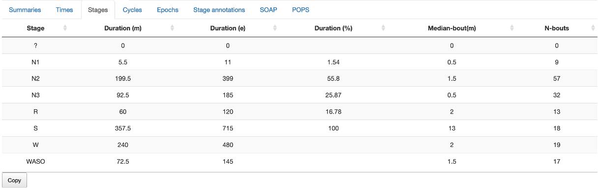
Stages
Stage duration (minutes, epochs and % of sleep) as well as the number
of bouts and the median bout length (minutes). Stages are defined as
N1, N2, N3, R and W. In addition, S is any sleep, WASO
is wake afetr sleep onset, and ? denotes unknown epochs.
Cycles
For NREM cycles inferred from the hypnogram, this sub-panel enumerates their start/stop times and extent of REM and NREM epochs.
Epochs
This sub-panel shows an epoch-level tabulation of sleep stages alongside some other key metrics from HYPNO: e.g. a marker of persistent sleep and WASO, as well as counts of elasped (cumulative) sleep.
Stage annotations
If the annotations present in the dataset aren't recognized by Luna
(i.e. are mapped to N1, N2, N3, ...) then the corresponding
labels can be selected explicitly here. Click Assign to recalculate
the hypnogram and metrics in this case. Often Luna will be able to
guess, e.g. Stage N2 is remapped to the standard label N2
internally.
SOAP
This sub-panel implements a simple single-channel instance of the SOAP model, described here. Select a channel (typically EEG, but it does not need to be - although it should have a minimal 50 Hz sample rate and be expected to vary with sleep stage) and then click Run SOAP. After a few seconds, a plot like the following will appear:
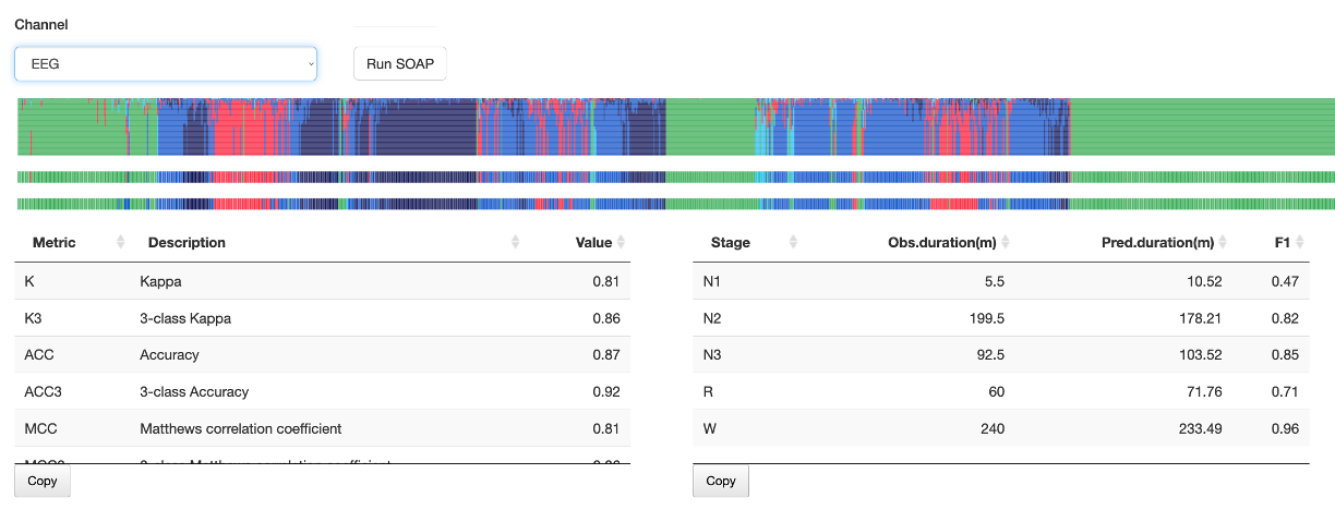
In all these plots, the x-axis corresponds to epochs - and will align
with the top spectrogram, hypnogram and mask plots. The upper plot
shows the posterior probabilities from SOAP (same color scheme as
above). The middle plot shows the most likely SOAP stage for each
epoch. The lower plot shows the original hypnogram in the same
condensed form. The tables beneath gives the SOAP kappa values and
estimates of stage duration, all as generated by the SOAP command.
In the SOAP context, low kappa values (e.g. less than 0.5) indicate
likely problems with the consistency of the signal and/or stage
annotations provided.
If no stage annotations are uploaded, then the SOAP module will not be available.
POPS
Moonlight currently supports two precomputed POPS models for automated sleep staging. POPS can be run whether or not any original stage annotations are present.
-
M1: single EEG model - expects a central EEG, contra-lateral mastoid referenced (although, in practice, the model is likely to be reasonably robust to other channels, e.g. frontal, or with linked-mastoid referencing used, etc) -
M2: similar toM1, except expecting two central EEGs (i.e.C3-M2andC4-M1typically). This uses POPS channel equivalance options to fit two single-EEG models and select the most confident predictions automatically (i.e. highest posterior for that epoch).
Both models expect signals to have been band-pass filtered 0.3 - 35 Hz
-- you can check the Pre-filter button if the signals have not been
filtered, and then Moonlight will perform the filtering on-the-fly.
(After running, filtered and normalized versions of the signal(s) used
will appear as new channels in the dataset, with _FLT and _NORM
extensions.)
Checking SHAP will produce SHAP information content scores for
different features used: this is an advanced feature that will not be
of use for most users and will slow down POPS also.
After clicking Run POPS, it can take around 5 to 10 seconds typically (depending on recording duration and original sample rate) to generate the predictions, which will appear as below:
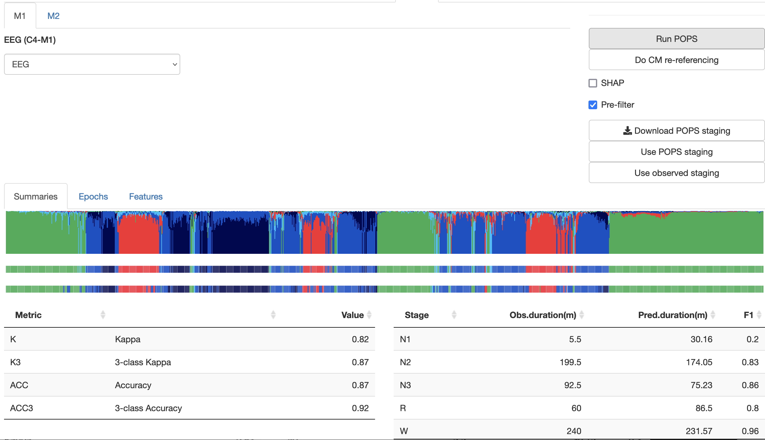
Above, the Summaries sub-panel shows a plot that is similar in structure to the SOAP plot described above (i.e. top two rows show POPS predictions, the bottom row shows any original staging). Beneath this, measures such as kappa and implied stage durations are shown, similar to SOAP.
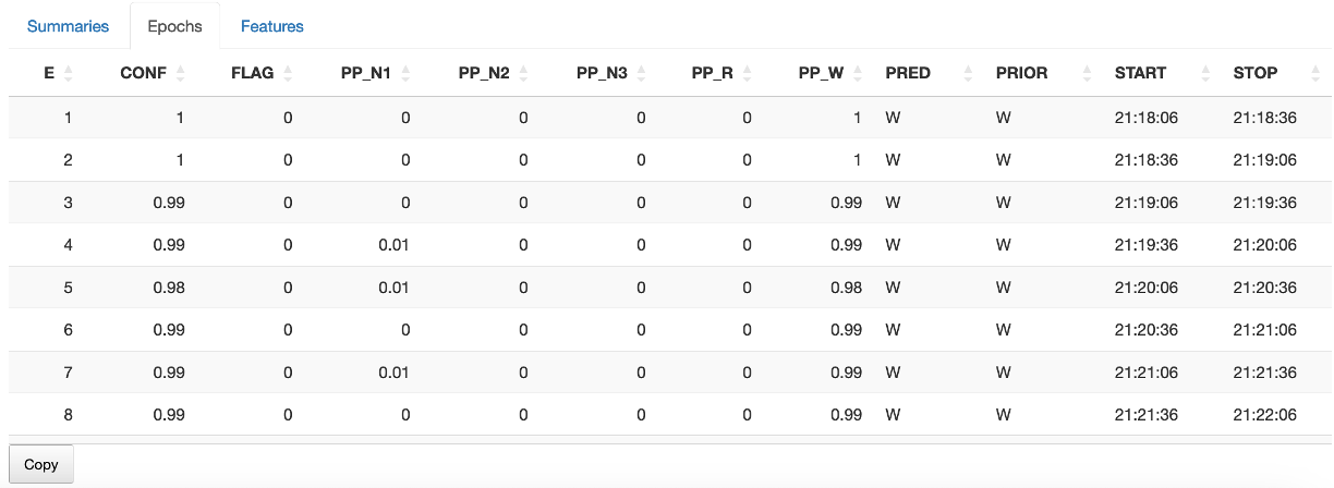
The Epochs sub-panel lists the predicted stages along with the posterior probabilties and the original stages (if present). This can be copied to the Clipboard and saved.
The POPS panel also contains buttons to:
-
automatically perform contra-lateral mastoid referencing on the selected central EEGs (assuming that either
A1andA2, orM1andM2exist) -
export the POPS staging to a file
-
two buttons to determine whether the primary hypnogram (i.e. Moonlight's awareness of sleep stage) should be based on any original staging (observed) versus the new POPS staging
Annots

This panel shows any annotations selected in the left panel Annotations list, in a whole-night plot (x-axis elapsed hours from EDF start), as below.
Summary
Benath the plot, the Summary sub-panel shows metrics for all annotations (not just those selected).
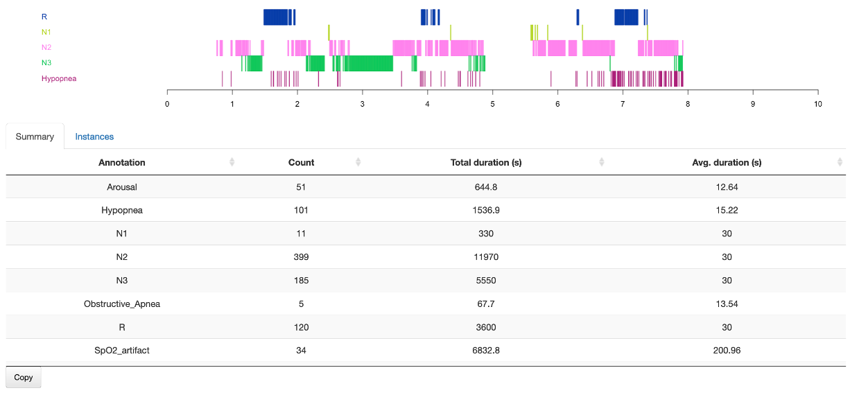
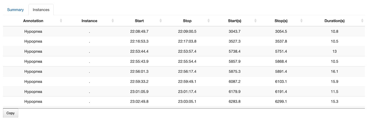
Instances
The Instances sub-panel shows the actual events for selected annotations only. This table can be sorted by different columns by clicking on the header; as with other Moonlight tables, it can be copied to the Clipboard.
Signals
For selected signals and annotations (from the left panel), this panel shows the raw data, e.g. here for several channels and annotations for a 30-second epoch (the default window size):
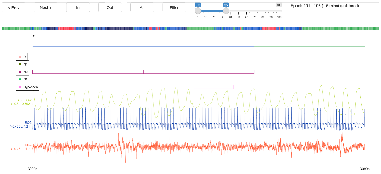
One can zoom out with the Out button (i.e. 1->3->5 epochs, etc) and back in with the In button. If the range is too large, raw signals will not be displayed.
You can click on the condensed hypnogram above the plot to move to that postiion (a small black dot under indicates the current location). You can also move the window forward and backward in time with the Next and Prev buttons. As noted above, you can also navigate around the recording by clicking on Listed annotations in the left panel. (To also see those annotations in the plot, they must also be selected in the upper Annotations list in the left panel.)
Filter toggles on/off a bandpass filter to all displayed signals (in the view only, this does not impact the underlying signal data).
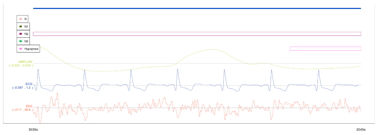
You can also select a region (holding down left mouse button) of the main window to zoom in - e.g. to look at only a few seconds of recording, as below:
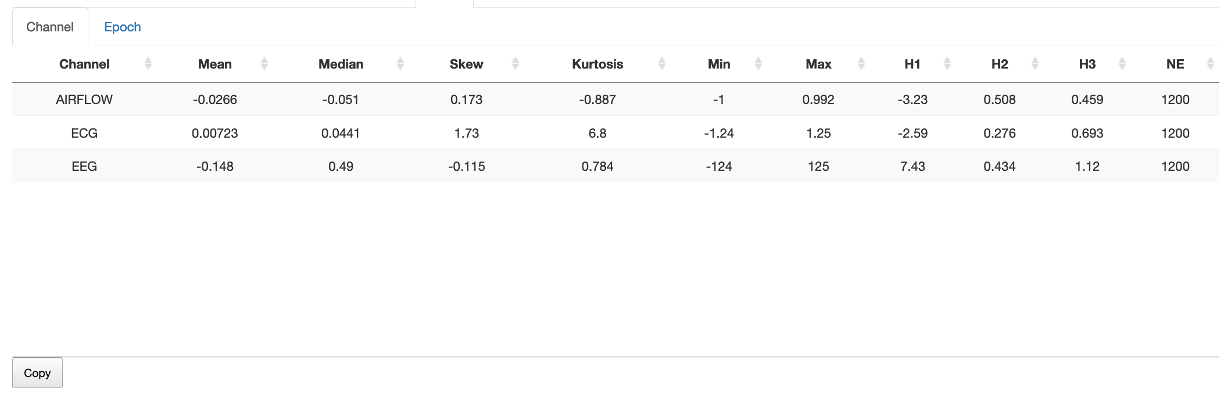
Stats

The Stats window takes the channels as selected in the left Channels tab, and for the current set of unmasked epochs calculates basic statistics (e.g. mean, min, max, etc).
Channel
Channel-level statistics are based on the median of epoch-level statistics, and are shown under the Stats/Channels sub-panel.
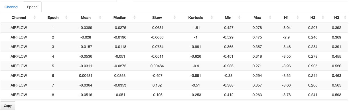
Epoch
Epoch-level statistics are also available under the Stats/Epochs sub-panel.
Time/frequency analyses
This tab contains a number of more advanced summaries and metrics.
Spectrogram
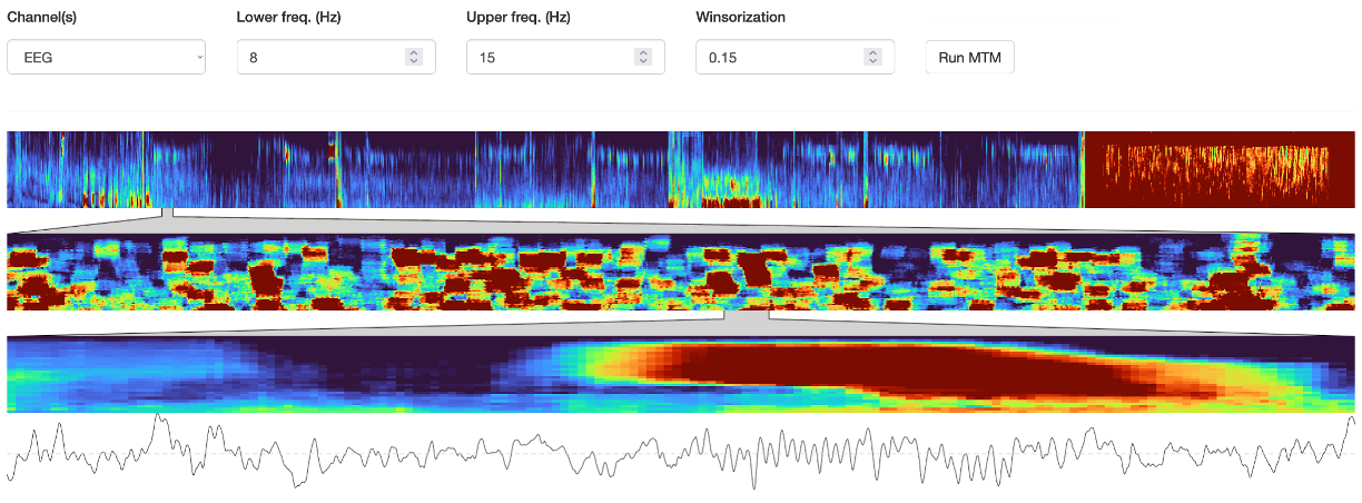
The Spectrogram sub-panel applies the MTM multi-taper spectrogram command. This is quite instence for a long/high-sample rate signal, i.e. it may take 5-10 seconds to complete. It is based not on the channel(s) in the left Channels box, but rather has its own Channel tab. You must hit Run MTM to generate the top level spectrogram.
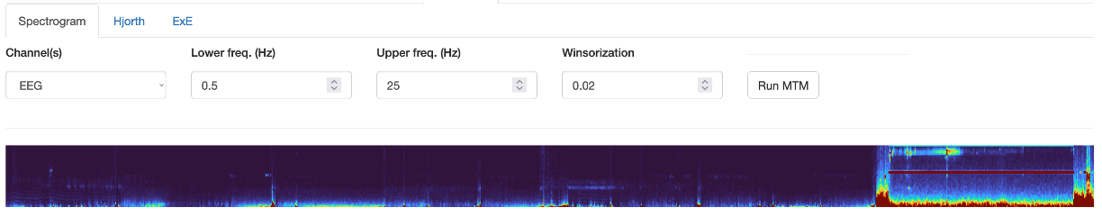
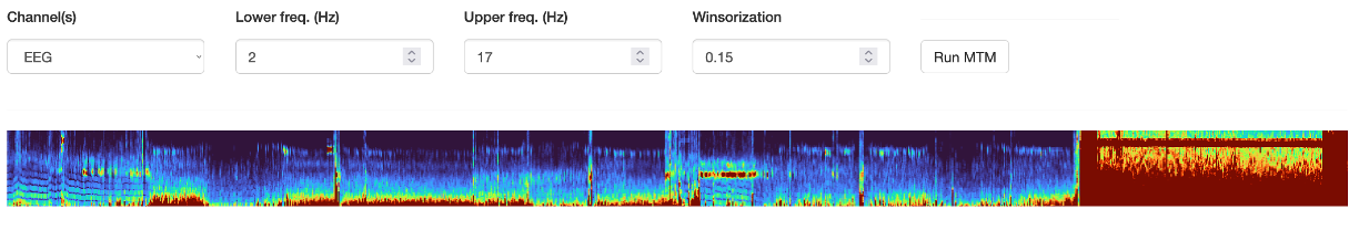
Note that the min/max frequency controls, as well as the winsorization (i.e. of the heatmap) can be altered after running the MTM - these modify the plot on-the-fly which can be useful for visualization. Here are the same data but with these parameters changed:
If you click anywhere within the top (whole-night) spectrogram, then (after a few seconds) two lower spectrograms will appear. The middle is a window of 1 minute, using a segment size of 6 seconds (with 0.25s increments) and tw parameter of 3. In contrast, the top spectrogram has a segment size of 30, no overlap, and tw of 15.
Clicking on the middle window re-centers the lower spectrogram, which is a 10-second window, using a segment size of 2.5s (increment 0.05 seconds) and tw of 5. The raw signal is also shown beneath for this interval:
The plot below shows the four windows:
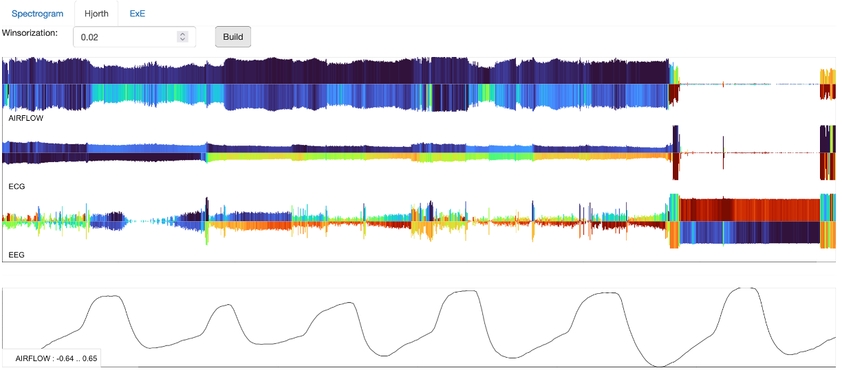
Hjorth
The Hjorth panel shows a series of so-called "Hjorth plots" for the signals selected by the left Channels tab.
Briefly, each line is one epoch, the x-axis is time across the night. The height of each bar is proportional to the first Hjorth parameter (activity / RMS). The color/heat of the top half of each line is proportional to the second Hjorth parameter, which basically tracks modal frequency. Thus blue means slower activity, reds mean faster activity. The lower half of each line is proportional to the third Hjorth parameter (complexity). Thus blues indicate signals that do not change markedly (in terms of their typical frequency of oscillation), whereas reds indicates more changeable/complex signals. A bottom panel will show the raw signal (30s epoch) for which channel/epoch the mouse is currently hovering over:
The plot below gives a three example epochs of raw signal (A, B and C) corresponding to various parts of the night for a single EEG.
-
A : both sides dark blue, meaning slower oscillations and consistent signals
-
B : a faster and more variable signal (i.e. reflecting interference)
-
C : a highly corrupt, clipped large-amplitude signal
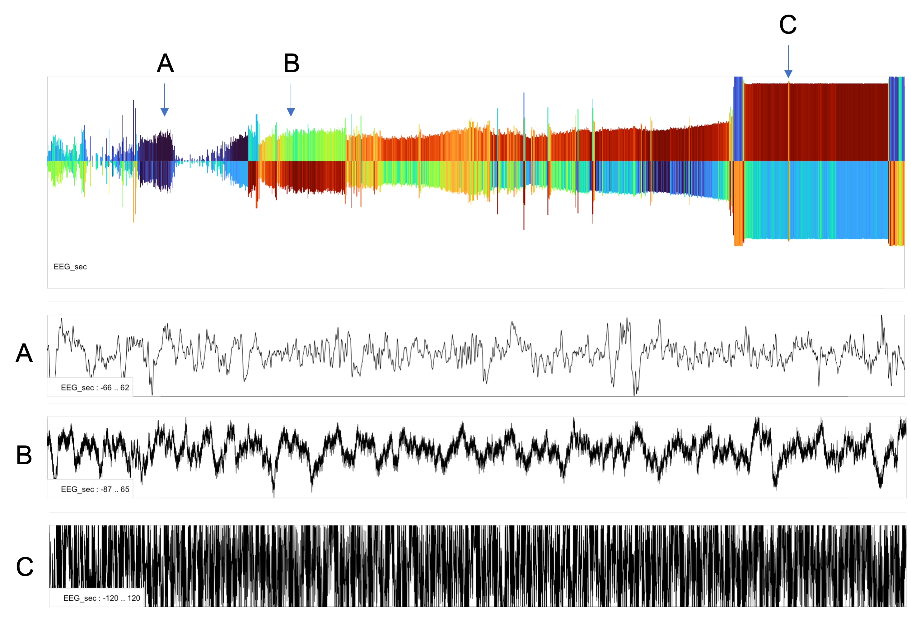
These types of plots can provide convenient summaries to show broad patterns of structure/gross artifacts in signls - in particular for signals where the typical time/frequency spectrograms may not be as convenient or readily interpretable (as they are for the EEG).
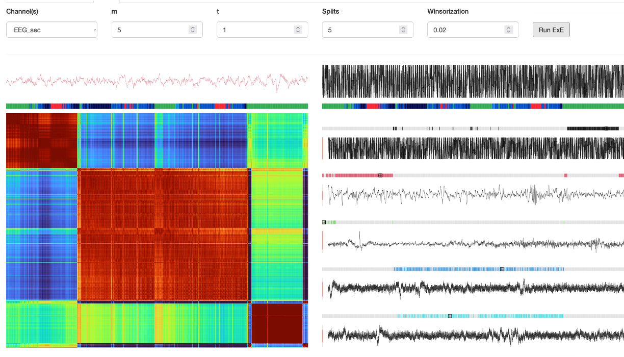
EXE
The EXE panel provides an implementation of the EXE representative command.
Select a single channel using the box in this panel (i.e. not the left Channels tab). The m, t and Splits parameters control
aspects of the clustering heuristic. After clicking Run ExE, you will see a) a heatmap of the epoch-by-epoch distance matrix on the left, b) five (by default)
exemplar epochs, along with an indication of the other epochs that are similar to it.
If you hover with the mouse over the heatmap, the corresponding raw signals will be shown at the top (left/right = row/column). Overall, this can provide a quick way to see the overall structure of a signal, and to zoom in on aberrant epochs, etc.
Manips

This panel provies a series of sub-panels to perform basic
manipulations of signals, most of which are self-explantory wrappers
around a corresponding Luna command (e.g. REFERENCE, FILTER,
MASK, RESAMPLE, etc)
Rereference
Reference channels specified selected in the left Channels box by the signal(s) in the Reference(s) box, then selecting Re-reference button. If more than one reference channel is selected, the average of those signals is taken first (i.e. to support linked-mastoid referencing, or common average referencing).
The CM-reference button will automatically look for the channels
C3, C4, F3, F4, O1 and O2 as well as M1/M2 (or
A1/A2) and perform the appropriate rereferencing, e.g. C3-M2,
C4-M1, etc.
Note that rereferencing does not change the label of the signal, so the user is responsible for tracking which signals have or have not been rereferenced.
Resample
The channels selected in the Channels box are resampled to sample rate as specified in the Sample rate (Hz) box (after clicking Resample)
Bandpass filter
Applies a FIR (Kaiser-window) bandpass filter to one or more signals selected in Channel(s).
Rename
Renames a single channel to a new label.
Drop
Drops one or more channels.
Copy
Copies a single channel and assigns a new label.
Transform
An advanced feature, this applies an arbitrary Eval transform expression to a single channel.
Mask
Applies a mask to the current data, by selecting
one or more annotations, indicating whether epochs with those
annotations should be included (i.e. MASK mask-ifnot) or excluded
(i.e. MASK mask-if) and then pressing the Set button. Here is an
example of a mask used to include on N2 epochs - after running, note how the track
at the top changes (just under the hypnogram) to reflect masked (gray) versus unmasked (orange)
epochs:
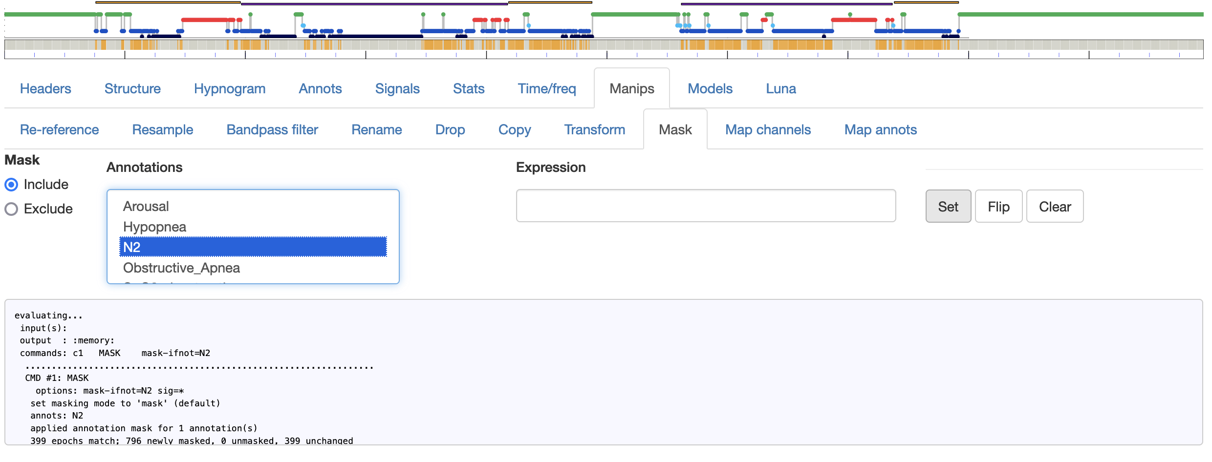
Alternative options (that do not use use the Mask or Annotations boxes are a) the Flip button, which simply flips the current mask, and b) the ability to write a generic mask argument (and then click Set to apply it).
Map channels
This is a wrapper around the CANONICAL command,
to map channel labels to a common standard. The current NSRR
canonical mapping file can be read in automatically via Insert NSRR defaults button.
Map annots
This is a wrapper around the REMAP command,
to map annotationns to a common standard. The current NSRR
annotation mapping file can be read in automatically via Insert NSRR defaults button.
Models

This tab is designed to host an hopefully growing set of predictive
models and other resources, including population norm data for common
sleep metrics. The models are initially based around Luna's
PREDICT command and the models therein.
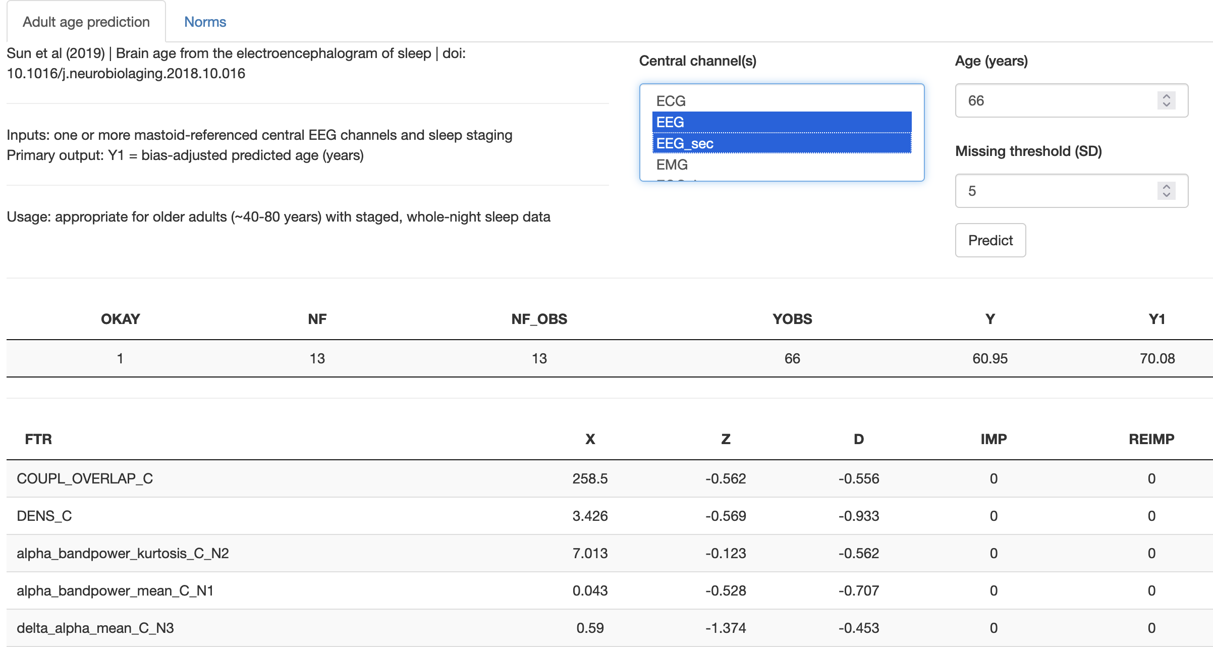
SUN2019: Adult age prediction
This is a wrapper around the PREDICT command for
the SUN2019 model to
predict adult "brain age" from the sleep EEG. It requires sleep
staging to be present (either from attached annotations, or previously
generated by the Moonlight/Luna POPS stager (see above).
The model assumes at least one central EEG: one or more central EEGs
can be selected from the Central channel(s) box. The individuals
observed (chronological) age should be specified in the top box.
Also, the threshold to flag outliers can be changed (default of 5 SD
units). After pressing Predict and waiting 10-20 seconds, the
output tables as shown below should be generated. The primary output
for this model is Y1, a bias-corrected estimate of biological/brain
age based on the sleep EEG. The difference between this and observed
age can be interpreted as a brain age index, see the above
manuscript for rationale and applications.
Processing many samples
If working with multiple recordings, this analysis can be automated by running directly on the command line as shown here.
We thank Drs. Sun, Westover and colleagues for sharing their work to support this implementation of their model.
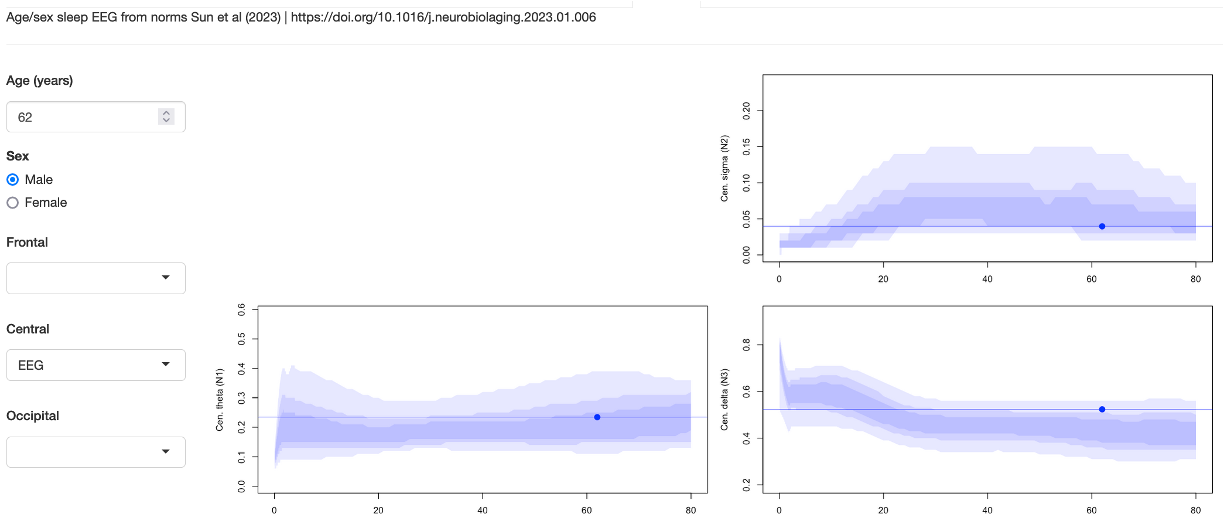
Population norms
This tab presents normative data for several sleep EEG metrics based on the publication of Sun et al. Given an attached EDF with staging and appropriate channels (frontal, central or occipital), it calculates several metrics in the same manner as the original paper, and then plots the results against the normative dataset as used in the above study.
We thank Drs. Sun, Westover and colleagues for sharing their work to support this implementation of their .
Luna
This panel allows arbitrary Luna commands to be executed on the currently attached EDF/annotation dataset, as well as providing a simple graphical viewer.
Limits of use and practical considerations
Although it can be convenient to use this feature to run specific one-off Luna commands in a flexible manner, this is not designed as a mature "front-end" for Luna. Learning to use Luna via the standard command-line is by far the best (most efficient and most reproducible) approach. Certain errors may not always be well caught by Moonlight, leading a a grayed-out screen: it can usually be more informative to see the whole console outputs from the command line. Alternatively, if running Moonlight locally via R or a Docker container, at least then one will be able to see Luna's console output directly, which can be helpful to assist debugging, etc.
Commands
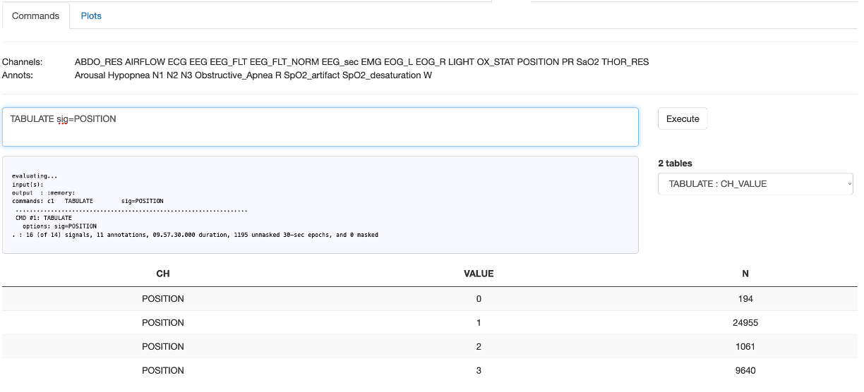
As one simple example, given an attached dataset (the Example dataset) here we run the TABULATE command, i.e.
equivalent to running
luna s.lst -o out.db -s ' TABULATE sig=POSITION '
assuming the s.lst pointed to the appropriate EDF/annotation pair. After clicking Execute,
the console output appers in the gray window, and any output tables (i.e. what would have been the
contents of out.db) are listed in the Tables tab. Selecting one of those will display it
in the table in the lower half of the panel:
As a second example, here we run a spectral analysis using the PSD command, running a multi-part command,
with commands separated either by new-lines, or by & symbols (i.e. the same as when using the standard command-line version of Luna):
MASK ifnot=N2
RE
PSD sig=EEG,EEG_sec spectrum dB max=65
which gives the output in the console:
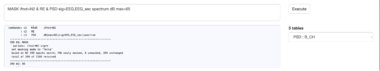
Looking at the first table: band power (i.e. outputs stratified by band (B) and channel (CH), we see this table:
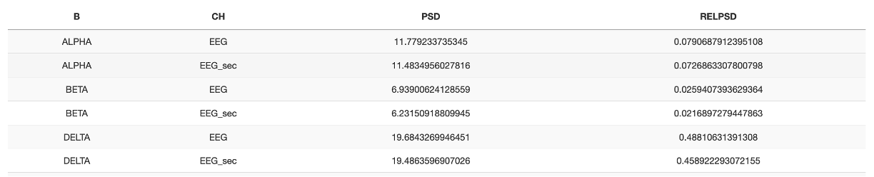
If outputs are better digested visually, one can either copy the table (at the bottom, each table with have a Copy button that copies it to the clipboard), or select the adjacent Plots subpanel after running a Luna command.
Plots
The Plots subpanel is designed to view any previously executed command from the Commands subpanel of Luna. Assuming the
above example has just been performed, we could select the power spectra which is the table stratified by both frequency bin (F)
and channel (F). See the main Luna documentation for a description of the outputs of each command.
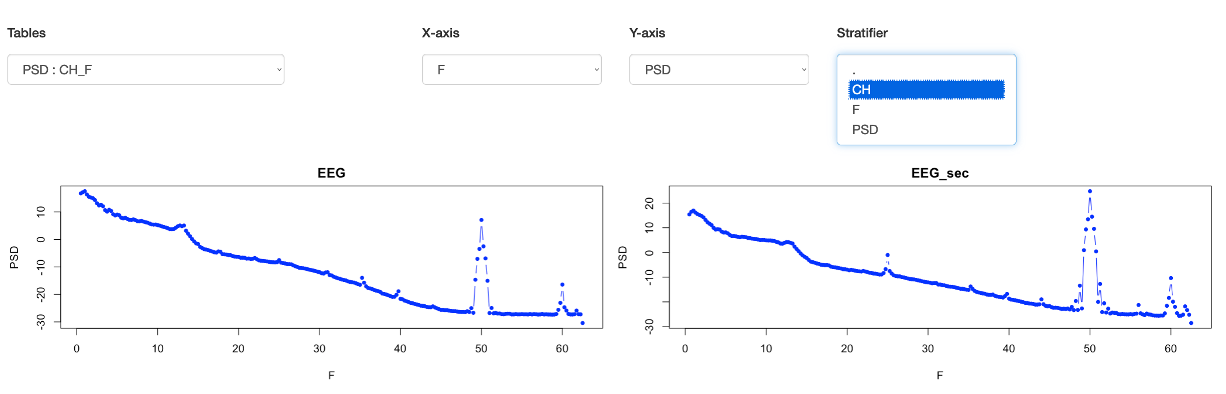
This tab provides a limited but potentially still convenient way to visualize some of the Luna outputs, in the form of scatter plots. To
see a power spectra emitted from the previous command, select F for the X-axis, and PSD for the Y-axis. You should then see the following
plots:
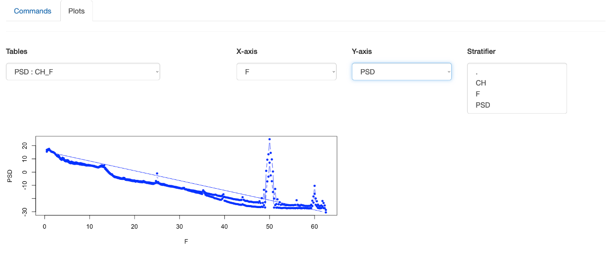
Here it is plotting values for both channels in the same plot, which is not what is desired (especially as it draws the line back between channels).
That is, remember that this Plot function is completely generic, and so does not understand what a particular plot should look like. We can however
select a Stratifier as channel (CH) which means that separate scatter plots will be made for each level (unique value) of the stratifier. This gives
two plots, one per channel, that show clearer results:
In this case, if you wanted to restrict the range of frequencies, you'd need to re-run the Luna command changing max to something higher or lower. Obviously for
more advanced/fine-grained manipulation, one should use a proper statistical/graphics package, however: this is designed for situations where a quick view of some
results can be of use.
This concludes our Moonlight tour