lunaR command reference
Attaching EDFs
lsl()
Imports a Luna sample-list into R
Syntax: sl <- lsl( file , path = "" )
-
fileis a required argument, giving the name of the sample-list file -
the optional
pathargument mirrors Luna'spathcommand-line option> sl <- lsl("s.lst") 3 observations in s.lst
Returns: a named-list representing the sample-list
-
names(sl)gives a list of IDs (i.e. first column) in the sample list:> names(sl) [1] "nsrr01" "nsrr02" "nsrr03" -
EDFandANNOTelements are the EDF and annotation filename(s) (sample lists can contain 0 or multiple annotation files):> str(sl) List of 3 $ nsrr01:List of 2 ..$ EDF : chr "edfs/learn-nsrr01.edf" ..$ ANNOT: chr "edfs/learn-nsrr01-profusion.xml" $ nsrr02:List of 2 ..$ EDF : chr "edfs/learn-nsrr02.edf" ..$ ANNOT: chr "edfs/learn-nsrr02-profusion.xml" $ nsrr03:List of 2 ..$ EDF : chr "edfs/learn-nsrr03.edf" ..$ ANNOT: chr "edfs/learn-nsrr03-profusion.xml"
lattach()
Loads an EDF and any associated annotation files from a
sample-list loaded by
lsl().
Syntax: lattach( sl , idx )
-
slis a sample-list as loaded bylsl() -
idxis either an integer number (in which case, it means to attach the EDF/annotations specified on that row of the sample-list), or a string value (in which case, it is interpreted as the ID of the individual/EDF to be attached)
Returns: no explicit return value: this command sets the in-memory EDF representation to reflect this EDF header/file, by calling ledf()
-
as well as attaching that EDF, this calls
lstat()to display some basic information about it; for example, to attach the second individual in the sample-list, one could use either:or:> lattach( sl , 2 ) nsrr02 : 14 signals, 10 annotations, of 09:57:30 duration> lattach( sl , "nsrr02" ) nsrr02 : 14 signals, 10 annotations, of 09:57:30 duration -
if the index or ID is out-of-range/not found, this command will give an error
Note
Unlike many R functions, lattach() does not return an
object that represents the data (i.e. the EDF). Rather, lunaR
is designed to operate on one EDF at a time; attached EDFs can be
displayed with the lstat() function. Attaching a new EDF
effectively detaches any previously attached EDF.
ledf()
Directly attaches an EDF
Syntax: ledf( edffile , id = "." , annots = character(0) )
-
edffileis a required filename for the to-be-attached EDF -
idis an optional ID that will be associated with this EDF -
annotsis an optional vector of one or more annotation filenames (.xml,.ftr,.annotor.eannotfiles, as described here)
Returns: Similar to lattach(), which is just a wrapper around the ledf() function
For example, here we use ledf() to directly achieve what we did with lattach() above:
> ledf("edfs/learn-nsrr02.edf" , "nsrr02" , "edfs/learn-nsrr02-profusion.xml" )
nsrr02 : 14 signals, 10 annotations, of 09:57:30 duration
lstat()
One line description to console of the currently-attached EDF
Syntax: lstat()
Returns: no explicit return values, other than output to console
This command is automatically called after each leval() or
lattach() command.
ldrop()
Detaches the current EDF
Syntax: ldrop()
Returns: no explicit return value
lrefresh()
Reattaches the currently attached EDF
Syntax: lrefresh()
Returns: no explicit return value
When lrefresh()-ing an attached EDF, any previous in-memory
modifications (i.e. from masking, filtering, or other manipulations)
are effectively reset.
Extracting data
lchs()
Returns the EDF channel names
Syntax: lchs()
Returns: a vector of channel names for the attached EDF:
> lchs()
 [1] "SaO2"     "PR"       "EEG(sec)" "ECG"      "EMG"      "EOG(L)"
 [7] "EOG(R)"   "EEG"      "AIRFLOW"  "THOR RES" "ABDO RES" "POSITION"
[13] "LIGHT"    "OX STAT"
ldata()
Returns a data frame of signals and annotations for requested epochs
Syntax: ldata( e , chs , annots = character(0) )
-
eis a required vector of 1-based epoch numbers corresponding to the current epoch numbering of the attached EDF -
chsis a required vector of channel names to be returned, i.e. as fromlchs(), all of which are required to have the same sampling rate -
annotsis an optional vector of annotation names to be returned, i.e. as fromlannots()
Returns: a data frame where each row is one sample point, containing the raw signal (and annotation) data and the following columns:
- epoch number
E - elapsed time since the start of the current first epoch
SEC - any signals, in alphabetical order, where column/variable names are the channel labels, potentially sanitized
if need be to remove special characters with an underscore (e.g. here
EEG(sec)becomesEEG_sec_): - any annotations, where
1and0indicate the presence/absence of that annotation at that time-point
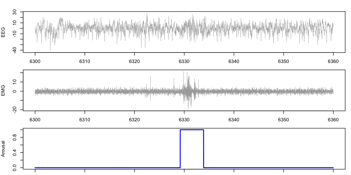
For example, here we request EEG and EMG channels for epochs 211 and
212, along with the arousal annotation from the tutorial dataset for
nsrr02:
d <- ldata( 211:212 , chs = c("EEG", "EMG") , annots = "arousal" )
> head(d)
    E      SEC       EEG        EMG arousal
1 211 6300.000 -4.411765 -2.8411765       0
2 211 6300.008 -5.392157  0.8647059       0
3 211 6300.016 -4.411765 -1.6058824       0
4 211 6300.024 -4.411765 -2.8411765       0
5 211 6300.032 -6.372549  1.3588235       0
6 211 6300.040 -6.372549 -0.1235294       0
par(mfcol=c(3,1),mar=c(1,4,2,1))
plot( d$SEC , d$EEG , type="l" , lwd=0.5 , col="darkgray",ylab="EEG")
plot( d$SEC , d$EMG , type="l" , lwd=0.5 , col="darkgray",ylab="EMG")
plot( d$SEC , d$arousal , type="l" , col="blue" , lwd=2,ylab="Arousal")
Warning
The following command would request all the data in an EDF (assuming that all channels have similar sampling rates) and all associated annotation information:
ne <- lepoch()
d <- ldata( 1:ne , lchs() , lannots() )
ldata()
may be large (i.e. too large), if many epochs, channels and/or annotations are requested...
If different channels have different sampling rates, use the RESAMPLE command to
resample one or more channels first. For example, if the EEG, ECG and EMG have different sampling rates, then this:
d <- ldata( 211:212 , c("EEG" , "ECG" , "EMG" ) , "arousal" )
Error in ldata(211:212, c("EEG", "ECG", "EMG"), "arousal") :
   requires uniform sampling rate across signals
We can first confirm the different sampling rates, by running
("evaluating") the Luna HEADERS
command with leval():
k <- leval( "HEADERS" )
lx():
lx( k , "HEADERS" , "CH" )
SR column shows sampling rates of 250, 125 and 125 Hz for ECG, EEG and EMG respectively:
         CH  DMAX   DMIN PDIM   PMAX    PMIN  SR
1  ABDO RES   127   -128       -1.00    1.00  10
2   AIRFLOW   127   -128       -1.00    1.00  10
3       ECG   127   -128   mV   1.25   -1.25 250
4       EEG   127   -128   uV 125.00 -125.00 125
5  EEG(sec)   127   -128   uV 125.00 -125.00 125
6       EMG   127   -128   uV  31.50  -31.50 125
7    EOG(L)   127   -128   uV 125.00 -125.00  50
8    EOG(R)   127   -128   uV 125.00 -125.00  50
9     LIGHT     1      0        1.00    0.00   1
10  OX STAT     3      0        3.00    0.00   1
11 POSITION     3      0        3.00    0.00   1
12       PR 32767 -32768  BPM 200.00    0.00   1
13     SaO2 32767 -32768    % 100.00    0.00   1
14 THOR RES   127   -128       -1.00    1.00  10
leval("RESAMPLE sig=ECG sr=125")
ldata() function will work: d <- ldata( 211:212 , c("EEG" , "ECG" , "EMG" ) , "arousal" )
> head(d)
    E      SEC       EEG        ECG        EMG arousal
1 211 6300.000 -4.411765 0.05936309 -2.8411765       0
2 211 6300.008 -5.392157 0.06401207  0.8647059       0
3 211 6300.016 -4.411765 0.06290266 -1.6058824       0
4 211 6300.024 -4.411765 0.05973290 -2.8411765       0
5 211 6300.032 -6.372549 0.06279700  1.3588235       0
6 211 6300.040 -6.372549 0.06448754 -0.1235294       0
ldata.intervals()
Returns raw signal and annotation data for requested intervals
Syntax: ldata.intervals( i , chs , annots = character(0) , w = 0 )
-
iis a required list of intervals (in seconds), e.g. as returned bylannots(annot) -
chsis a required vector of channel names to be returned, i.e. as from lchs(), all of which are required to have the same sampling rate is a required vector of channel names -
annotsis an optional vector of annotation names to be returned, i.e. as fromlannots() -
wis an optional window (in seconds) the specifies whether the returned region should also contain a window of up towseconds each side of the specified interval(s). For example, if the intervals represented individual sleep spindles, then addingw=10would return windows of approximately 20 seconds, with the spindle centered in the middle.
Returns: a data frame where each row is one sample point,
containing the raw signal (and annotation) data. See the description
of ldata's output for more information. columns
This command is effectively the same as ldata() except
that the regions of interest are specified as intervals rather than
in terms of epoch numbers. Intervals are defined as half-open
intervals [a,b), meaning all sample-points equal to or greater
than a, but less than b.
Annotations
lannots()
Returns a vector of annotation class names, _or all intervals for a given annotation class_
Syntax: lannots( a = "" )
ais an optional annotation name, i.e. matching one value returned bylannots()
Returns: if no specific annotation is specified, this returns a vector of annotation class names for the attached dataset:
> lannots()
 [1] "NREM1"             "NREM2"             "NREM3"
 [4] "REM"               "apnea_obstructive" "arousal"
 [7] "artifact_SpO2"     "desat"             "hypopnea"
[10] "wake"
Alternatively, if a is a valid annotation class name for that individual, this function instead returns a list of intervals (two-element vectors)
for each instance of that annotation class:
head( lannots("wake") )
[[1]]
[1]  0 30

[[2]]
[1] 30 60

[[3]]
[1] 60 90

[[4]]
[1]  90 120

[[5]]
[1] 120 150

[[6]]
[1] 150 180
lepoch()
Sets epochs for the current EDF
Syntax: lepoch( dur=30 , inc=dur )
-
the epoch duration (
dur) defaults to 30 seconds iflepoch()is called with no arguments -
the epoch increment (
inc) defaults todur(i.e. non-overlapping epochs) unless otherwise specified
Returns: when assigned to another variable, this function returns the number of epochs set:
> ne <- lepoch()
evaluating...
nsrr02 : 14 signals, 10 annotations, of 09:57:30 duration, 1195 unmasked 30-sec epochs, and 0 masked
> ne
[1] 1195
Note
lepoch(30) is identical to using the leval() function to evaluate/execute an EPOCH command:
leval( "EPOCH dur=30" )
letable()
Returns an epoch-level data frame with time, mask and annotation information
Syntax: d <- letable( annots = character(0) )
annotsis an optional vector of annotation class names, as returned bylannots()
Returns: a data frame with at least six columns:
Eepoch number of the current unmasked datasetSECelapsed seconds for the current unmasked datasetE1epoch number for the original datasetSEC1elapsed seconds based on the original dataHMSclock-time for epoch startMflag to indicate whether this epoch is masked (1) or not (0)- any additional columns will be labeled based on the specified annotations, with a flag (
1or0) to indicate whether or not that epoch contains at least one of that annotation class
For example, to look at the first few epochs:
d <- letable( annots=c("wake" , "NREM1" , "NREM2" ) )
dim(d):
[1] 1195 9
head(d)
  E SEC E1 SEC1      HMS M NREM1 NREM2 wake
1 1   0  1    0 21:18:06 0     0     0    1
2 2  30  2   30 21:18:36 0     0     0    1
3 3  60  3   60 21:19:06 0     0     0    1
4 4  90  4   90 21:19:36 0     0     0    1
5 5 120  5  120 21:20:06 0     0     0    1
6 6 150  6  150 21:20:36 0     0     0    1
Using leval(), we can set a
mask, for example, to mask everything except
epochs 2 to 5:
leval( "MASK epoch=2-5" )
evaluating...
nsrr02 : 14 signals, 10 annotations, of 09:57:30 duration, 4 unmasked 30-sec epochs, and 1191 masked
This masking would then be evident in the epoch-table (run here without additional annotation columns):
> head( letable() )
   E SEC E0 SEC0      HMS M
1 NA  NA  1    0 21:18:06 1
2  1   0  2   30 21:18:36 0
3  2  30  3   60 21:19:06 0
4  3  60  4   90 21:19:36 0
5  4  90  5  120 21:20:06 0
6 NA  NA  6  150 21:20:36 1
That is, the M column indicates which epochs are masked with a 1;
the current epoch-numbering E (of the 4 unmasked epochs) therefore
starts are what was epoch number E1 of 2 up to epoch number 5. (The
leftmost column of numbers are just the row numbers for the data
frame.) One might next restructure the dataset, i.e. to actually remove
masked epochs:
leval( "RESTRUCTURE" )
evaluating...
nsrr02 : 15 signals, 10 annotations, of 00:02:00 duration, 4 unmasked 30-sec epochs, and 0 masked
letable()
  E SEC E0 SEC0      HMS M
1 1   0  2   30 21:18:36 0
2 2  30  3   60 21:19:06 0
3 3  60  4   90 21:19:36 0
4 4  90  5  120 21:20:06 0
lrefresh() the dataset however:
lrefresh()
nsrr02 : 14 signals, 10 annotations, of 09:57:30 duration
lepoch()
evaluating...
nsrr02 : 14 signals, 10 annotations, of 09:57:30 duration, 1195 unmasked 30-sec epochs, and 0 masked
> head( letable() )
  E SEC E0 SEC0      HMS M
1 1   0  1    0 21:18:06 0
2 2  30  2   30 21:18:36 0
3 3  60  3   60 21:19:06 0
4 4  90  4   90 21:19:36 0
5 5 120  5  120 21:20:06 0
6 6 150  6  150 21:20:36 0
lstages()
Returns a vector of sleep stages based on annotation data
Syntax: lstages()
Returns: this convenience function gives a vector of sleep stage labels, i.e. based on attached annotations. For NSRR and other data, Luna expects a standard format for stage names, although this can be modified. See here for more information. This command is identical to running:
leval("STAGE")$STAGE$E$STAGE
ladd.annot()
Adds new annotations to the currently attached EDF given an interval list
Syntax: ladd.annot( annot , intervals )
annotis a required annotation class name for the new annotationintervalsis a required list of intervals, in the same format as returned bylannots(annot)
Returns: no explicit return value
Added annotations will be visible with subsequent lannots() commands.
ladd.annot.file()
Adds new annotations to the currently attached EDF from a file
Syntax: ladd.annot.file( a )
ais a required annotation file name
Returns: no explicit return value
This command is similar to specifying an annotation file in a sample-list. Epoch annotation (.eannot) files must match the attached EDF in terms of the number of current epochs.
Running Luna commands
leval()
Evaluates a set of Luna commands for the current attached dataset
Syntax: k <- leval( command )
-
commandis a single string or character vector of Luna commands, or the return value oflcmd() -
as for commands following
-swhen using the command line version of luna, different commands must be separated by a&character -
alternatively, multiple commands can be specified as elements of a vector: that is, the following are identical:
k <- leval( "MASK ifnot=NREM2 & RE & PSD" )cmds <- c( "MASK ifnot=NREM2" , "RE" , "PSD" ) k <- leval( cmds )
Returns: a list of data-frames, in which list items are commands
and sub-items are output strata, i.e. a similar organization to
destrat output (lunout) databases. The
lx() function is designed to facilitate working with these lists, as
shown below.
For example, here we estimate the PSD for all N2 epochs (for tutorial individual nsrr02):
k <- leval( "EPOCH & MASK ifnot=NREM2 & RE & PSD epoch spectrum sig=EEG" )
The overall structure of the returned list (k) can be viewed with R's str() function:
> str(k)
List of 4
 $ EPOCH:List of 1
  ..$ BL:'data.frame':  1 obs. of  3 variables:
  .. ..$ DUR: num 30
  .. ..$ INC: num 30
  .. ..$ NE : num 399
 $ MASK :List of 1
  ..$ EPOCH_MASK:'data.frame':  1 obs. of  7 variables:
  .. ..$ EPOCH_MASK  : chr "NREM2"
  .. ..$ N_MASK_SET  : num 0
  .. ..$ N_MASK_UNSET: num 0
  .. ..$ N_MATCHES   : num 399
  .. ..$ N_RETAINED  : num 399
  .. ..$ N_TOTAL     : num 399
  .. ..$ N_UNCHANGED : num 399
 $ PSD  :List of 4
  ..$ CH    :'data.frame':  1 obs. of  2 variables:
  .. ..$ CH: chr "EEG"
  .. ..$ NE: num 399
  ..$ B_CH  :'data.frame':  10 obs. of  4 variables:
  .. ..$ B     : chr [1:10] "ALPHA" "BETA" "DELTA" "FAST_SIGMA" ...
  .. ..$ CH    : chr [1:10] "EEG" "EEG" "EEG" "EEG" ...
  .. ..$ PSD   : num [1:10] 15.65 5.12 108.24 3.08 5.4 ...
  .. ..$ RELPSD: num [1:10] 0.0709 0.0232 0.4903 0.0139 0.0245 ...
  ..$ CH_F  :'data.frame':  41 obs. of  3 variables:
  .. ..$ CH : chr [1:41] "EEG" "EEG" "EEG" "EEG" ...
  .. ..$ F  : num [1:41] 0 0.25 0.75 1.25 1.75 2.25 2.75 3.25 3.75 4.25 ...
  .. ..$ PSD: num [1:41] 15.2 77.7 70.6 45.9 37.4 ...
  ..$ B_CH_E:'data.frame':    3990 obs. of  5 variables:
  .. ..$ B     : chr [1:3990] "ALPHA" "ALPHA" "ALPHA" "ALPHA" ...
  .. ..$ CH    : chr [1:3990] "EEG" "EEG" "EEG" "EEG" ...
  .. ..$ E     : int [1:3990] 92 93 98 99 100 101 102 118 119 120 ...
  .. ..$ PSD   : num [1:3990] 29.5 37.5 33.5 22.7 17.8 ...
  .. ..$ RELPSD: num [1:3990] 0.159 0.131 0.12 0.141 0.1 ...
 $ RE   :List of 1
  ..$ BL:'data.frame':  1 obs. of  4 variables:
  .. ..$ DUR1: num 11970
  .. ..$ DUR2: num 11970
  .. ..$ NR1 : num 11970
  .. ..$ NR2 : num 11970
That is, this performs exactly the same set of operations as the following command-line lunaC statement (i.e. when working with the same tutorial dataset):
luna s.lst 2 -o out.db -s "EPOCH & MASK ifnot=NREM2 & RE & PSD sig=EEG epoch spectrum"
The contents of the resulting out.db file from the lunaC command
will be similar to the k list in R (except baseline strata are
represented by BL rather than a period (.) character):
--------------------------------------------------------------------------------
distinct strata group(s):
  commands      : factors           : levels        : variables
----------------:-------------------:---------------:---------------------------
  [EPOCH]       : .                 : 1 level(s)    : DUR INC NE
                :                   :               :
  [RE]          : .                 : 1 level(s)    : DUR1 DUR2 NR1 NR2
                :                   :               :
  [PSD]         : CH                : 1 level(s)    : NE
                :                   :               :
  [MASK]        : EPOCH_MASK        : 1 level(s)    : N_MASK_SET N_MASK_UNSET N_MATCHES
                :                   :               : N_RETAINED N_TOTAL N_UNCHANGED
                :                   :               :
                :                   :               :
  [PSD]         : F CH              : 41 level(s)   : PSD
                :                   :               :
  [PSD]         : B CH              : 10 level(s)   : PSD RELPSD
                :                   :               :
  [PSD]         : E B CH            : (...)         : PSD RELPSD
                :                   :               :
----------------:-------------------:---------------:---------------------------
In R, the lx() function provides a concise summary of
the returned list (k in this case), which shows the four commands,
and the strata (or virtual tables) associated with each command's
output:
lx(k)
EPOCH : BL
MASK : EPOCH_MASK
PSD : CH B_CH CH_F B_CH_E
RE : BL
Note how the factors that define each virtual table (e.g. B and
CH) are concatenated together (e.g. B_CH). To extract the actual
results from a particular strata, e.g. for PSD results defined by
both spectral band (B) and channel (CH), we can use an augmented
version of lx(), with extra parameters:
lx(k,"PSD","B","CH")
            B  CH        PSD     RELPSD
1       ALPHA EEG  15.654212 0.07091026
2        BETA EEG   5.123496 0.02320835
3       DELTA EEG 108.239902 0.49030380
4  FAST_SIGMA EEG   3.078775 0.01394620
5       GAMMA EEG   5.403482 0.02447663
6       SIGMA EEG   8.440213 0.03823237
7        SLOW EEG  38.865512 0.17605253
8  SLOW_SIGMA EEG   5.361438 0.02428618
9       THETA EEG  31.416015 0.14230789
10      TOTAL EEG 220.760887 1.00000000
To confirm that similar results were obtained from lunaC, this is
equivalent to running the following destrat command (nb. output is
formatted differently, e.g. in lunaR all factor levels are sorted
alphabetically):
destrat out.db +PSD -r B CH
ID       B           CH     PSD          RELPSD
nsrr02   SLOW        EEG    38.86551     0.17605
nsrr02   DELTA       EEG    108.23990    0.49030
nsrr02   THETA       EEG    31.41602     0.14231
nsrr02   ALPHA       EEG    15.65421     0.07091
nsrr02   SIGMA       EEG    8.44021      0.03823
nsrr02   SLOW_SIGMA  EEG    5.36144      0.02429
nsrr02   FAST_SIGMA  EEG    3.07877      0.01395
nsrr02   BETA        EEG    5.12350      0.02321
nsrr02   GAMMA       EEG    5.40348      0.02448
nsrr02   TOTAL       EEG    220.76089    1.00000
Note
Each time lunaC (the command-line version of Luna) is run, it is
applied to a "fresh" version of the data, i.e. the EDF on disk.
In contrast, leval() statements within the same R session will
have cumulative effects on the internal EDF, which will persist
until either lrefresh() is called to re-attach a
"fresh" version of the data, or it is dropped (with
ldrop()), or a different EDF is attached (with
lattach() or ledf()).
In other words, if the EDF file has 14 signals, then running lunaC
from the command line will still show 14 signals from
the second DESC command:
luna s.lst 2 -s "SIGNALS keep=EEG"
luna s.lst 2 -s "DESC"
In R, with the same EDF [lattach()](#lattach()-ed, the second DESC statement
will report only 1 signal (not 14):
leval( "SIGNALS keep=EEG" )
leval( "DESC" )
leval() statements are made, they are really equivalent to the following command line (i.e. which would also show that only 1 signal is present from DESC):
luna s.lst 2 -s "SIGNALS keep=EEG & DESC"
lcmd()
Reads Luna commands from a file
Syntax: lcmd( filename )
filenameis a required parameter, the name of the file to read
Returns: a vector of Luna commands, parsed from the command
file in a manner that is suitable for
leval() (and leval.project(). That
is, blank lines and comments (starting with %) are stripped away,
and multi-line statements are concatenated into a single line.
Typical use will be in the form:
k <- leval( lcmd( "/path/to/command.txt" ) )
leval.project()
Evaluates a Luna commands for all individuals in a sample-list
Syntax: leval.project( sl , command )
-
slis a required sample-list, as returned bylsl() -
commandis a single string or character vector of Luna commands, or the return value oflcmd()
Returns: the same list-of-data-frames as returned by
leval(), except each data-frame will now contain all
individuals in the project specified by sample list sl.
The leval.project() function basically works in the same way as lunaC. In other words,
the following:
k <- leval.project( lsl( "s.lst" ) , lcmd( "cmd.txt" ) )
luna s.lst -o out.db < cmd.txt
Indeed, you can subsequently read out.db into lunaR with the
ldb() function:
k2 <- ldb( "out.db" )
k and k2 are effectively identical.
Differences between leval() and leval.project()
Unlike leval(), the leval.project() function
attaches and then drops each EDF in the sample list, iteratively. This means that
any changes to the internal EDFs will not persist across different runs of leval.project() in the way
they do for leval(). In other words, if the first individual from s.lst is currently attached, then:
leval( "MASK ifnot=NREM1" )
leval( "MASK ifnot=NREM2" )
leval( "RE" )
leval( "PSD" )
luna s.lst 1 -s "MASK ifnot=NREM1 && MASK ifnot=NREM2 && RE && PSD"
leval.project( sl , "MASK ifnot=NREM1" )
leval.project( sl , "MASK ifnot=NREM2" )
leval.project( sl , "RE" )
leval.project( sl , "PSD" )
luna s.lst -s "MASK ifnot=NREM1"
luna s.lst -s "MASK ifnot=NREM2"
luna s.lst -s "RE"
luna s.lst -s "PSD"
literate()
Applies an arbitrary R function to each epoch
Syntax: literate( func , chs = lchs() , annots= lannots() , by.annot = character(0) , w = 0 )
funcis a required argument, which specifies a user-defined R function to be evaluated per-epoch (or per interval)- optionally,
chsis a vector of channel names to be extracted each epoch (by default, all are) - optionally,
annotsis a vector of annotation class names to be extracted each epoch (by default, all are) - optionally,
by.annotis a single annotation class name, in which case this function iterates over each instance of that annotation class, rather than each epoch - optionally,
wis a window (in seconds) added to each annotation instance, ifby.annothas been specified
Returns: no explicit return value: it is expected that the user
will craft the function func in a way to capture relevant
information
The literate() function aims to make lunaR somewhat extensible, by
allowing users to add their own functions, in a way that can take
advantage of the masking, filtering and intersection with annotation
data afforded by the core Luna engine. This function iterates either
one epoch or one interval (based on annotation instances) at a
time. If not based on annotation intervals (with by.annot), you
therefore need to set epochs (with with lepoch()) prior
to running literate().
For each epoch, lunaR creates a data-frame in the same format as
returned by the ldata() and
ldata.intervals() commands, and passes it to the
user-defined function specified in literate(). The user's function
must therefore a) know what input to expect, b) appropriately perform
any calculations and c) store results as desired.
As an example: say that Luna did not have the root mean square (RMS)
function available in SIGSTATS, but
we wanted to calculate it, epoch-by-epoch for nsrr02's EEG channel.
We can define a new R function rms() that takes a vector x and
returns the root mean square:
rms <- function(x) { sqrt(mean(x^2)) }
> rms( c( 1,2,3 ) )
[1] 2.160247
> sqrt( ( 1 + 4 + 9 ) / 3 )
[1] 2.160247
We cannot just pass this function to literate(), as it would not
appropriately handle the data-frames passed by literate() and, also, it
does not save any output. In this case, we must therefore create a wrapper
function f1(), to call rms() appropriately and save the output, in
a new R environment called
e.
That is, we first create a new environment, which contains an empty
vector ret in which we can store the epoch-per-epoch output:
e <- new.env()
e$ret <- numeric()
Next, we create the wrapper function f1(), to take the EEG
variable from its input, x, where x will be a data-frame with the
same format as generated by ldata():
f1 <- function(x) { epoch = x$E[1]; e$ret[ epoch ] <- rms( x$EEG - mean(x$EEG) ) }
For correspondence with Luna's SIGSTATS, the above function also
mean-centers the signal prior to calculating the RMS. The f1()
function takes the epoch number as the first element in the E field, and
populates that entry of e$ret with the RMS. Naturally, there are
many other -- and probably better -- ways of achieving this goal using
R, but for now the above approach should work.
If the attached EDF is not already epoched, you must run lepoch()
first, as by default literate() iterates over epochs. We can then
call literate(), and pass f1() as the function to call:
literate( f1 , chs="EEG" , annots="" )
........................................ 40 epochs
........................................ 80 epochs
........................................ 120 epochs
........................................ 160 epochs
........................................ 200 epochs
........................................ 240 epochs
........................................ 280 epochs
........................................ 320 epochs
........................................ 360 epochs
........................................ 400 epochs
........................................ 440 epochs
........................................ 480 epochs
........................................ 520 epochs
........................................ 560 epochs
........................................ 600 epochs
........................................ 640 epochs
........................................ 680 epochs
........................................ 720 epochs
........................................ 760 epochs
........................................ 800 epochs
........................................ 840 epochs
........................................ 880 epochs
........................................ 920 epochs
........................................ 960 epochs
........................................ 1000 epochs
........................................ 1040 epochs
........................................ 1080 epochs
........................................ 1120 epochs
........................................ 1160 epochs
................................... 1195 epochs, done
When this completes, there will be a newly-populated ret vector in the e environment:
> ls(e)
[1] "ret"
> head( e$ret )
[1] 11.97071 15.87002 12.46824 11.34265 12.28683 15.23002
To confirm this worked as expected, we can compare this to the
epoch-level output from the actual SIGSTATS command, which
calculates RMS (it also mean-centers each epoch prior to calculating
this and Hjorth parameters, etc, which is why we added the step in
f1() above). Using leval():
> k <- leval( "SIGSTATS epoch sig=EEG" )
> lx(k)
SIGSTATS : CH CH_E
> head( k$SIGSTATS$CH_E )
   CH E        CLIP       H1        H2        H3      RMS
1 EEG 1 0.000000000 143.2979 0.6700231 0.9386154 11.97071
2 EEG 2 0.000000000 251.8576 0.6238226 1.0286470 15.87002
3 EEG 3 0.000000000 155.4571 0.6035006 0.9897814 12.46824
4 EEG 4 0.000000000 128.6557 0.5528684 0.9927338 11.34265
5 EEG 5 0.000266809 150.9661 0.4067636 0.9666429 12.28683
6 EEG 6 0.000000000 231.9535 0.4652896 1.0428972 15.23002
RMS field from the above table:
luna.rms <- k$SIGSTATS$CH_E$RMS
literate() approach:
> all.equal( e$ret ,  k$SIGSTATS$CH_E$RMS )
[1] TRUE
Working with output
ldb()
Imports the contents of a lunout database
Syntax: k <- ldb( dbfilename , id = "" )
-
dbfilenameis the name of a lunout database -
optionally, if
idis a vector of individual/EDF IDs, then only these individuals will be extracted from the database
Returns: a named-list R object, in the same format as
leval()
For example, based on the tutorial data, consider
the following out.db file, which will contain results for three
individuals:
luna s.lst -o out.db -s "HEADERS"
In R, this file can be directly imported with ldb():
k <- ldb( "out.db" )
read data on 3 individuals
The returned list k now contains the information from out.db:
k
$HEADERS
$HEADERS$BL
      ID    NR NS REC.DUR TOT.DUR.HMS TOT.DUR.SEC
1 nsrr01 40920 14       1    11:22:00       40920
2 nsrr02 35850 14       1    09:57:30       35850
3 nsrr03 40920 14       1    11:22:00       40920

$HEADERS$CH
       ID       CH  DMAX   DMIN PDIM   PMAX    PMIN  SR
1  nsrr01 ABDO RES   127   -128       -1.00    1.00  10
2  nsrr02 ABDO RES   127   -128       -1.00    1.00  10
3  nsrr03 ABDO RES   127   -128       -1.00    1.00  10
4  nsrr01  AIRFLOW   127   -128       -1.00    1.00  10
5  nsrr02  AIRFLOW   127   -128       -1.00    1.00  10
6  nsrr03  AIRFLOW   127   -128       -1.00    1.00  10
7  nsrr01      ECG   127   -128   mV   1.25   -1.25 250
8  nsrr02      ECG   127   -128   mV   1.25   -1.25 250
9  nsrr03      ECG   127   -128   mV   1.25   -1.25 250
10 nsrr01      EEG   127   -128   uV 125.00 -125.00 125
11 nsrr02      EEG   127   -128   uV 125.00 -125.00 125
12 nsrr03      EEG   127   -128   uV 125.00 -125.00 125
... (cont'd) ...
As noted, the returned value is in the same format as is generated by
leval() and can be parsed with lx() and
lid().
lx()
Extract the levels/table(s) from an output list generated by leval(), leval.project() or ldb()
Syntax: d <- lx( lst , cmd , f , ... )
-
lstis a required named-list object, as generated byleval(),leval.project()orldb() -
optionally,
cmdnames a command (i.e. a first-level item oflst) -
optionally,
f(and all other following arguments:...) specify a specific strata to return (i.e. the second-level items oflst)
Returns: depending on the arguments given, either a data-frame, a list of data-frames or only a message to the console
For example, consider the example given above for the
leval() command, which performed power spectral density
estimation for the EEG channel, for all N2 sleep for the nsrr02
individual. Assuming you have the tutorial data in
the current folder, this is generated as follows:
sl <- lsl( "s.lst" )
lattach( sl , 2 )
k <- leval( "EPOCH & MASK ifnot=NREM2 & RE & PSD epoch spectrum sig=EEG" )
lx() to work with this returned list k. In the first form, lx() just returns a message to the console
that lists the commands and strata present:
lx(k)
EPOCH : BL
MASK : EPOCH_MASK
PSD : CH B_CH CH_F B_CH_E
RE : BL
Note that lunaR appends factor names together with an underscore
(_) character (after sorting them in alphabetical order).
Therefore, B_CH means output that is stratified by both band (B)
and channel (CH) and will therefore contain these two variables in
the associated data-frame.
The above output corresponds to the structure as evident in the
str() function, e.g.:
str( k , max.level=2 )
List of 4
 $ EPOCH:List of 1
  ..$ BL:'data.frame':  1 obs. of  4 variables:
 $ MASK :List of 1
  ..$ EPOCH_MASK:'data.frame':  1 obs. of  8 variables:
 $ PSD  :List of 4
  ..$ CH    :'data.frame':  1 obs. of  3 variables:
  ..$ B_CH  :'data.frame':  10 obs. of  5 variables:
  ..$ CH_F  :'data.frame':  41 obs. of  4 variables:
  ..$ B_CH_E:'data.frame':  3990 obs. of  6 variables:
 $ RE   :List of 1
  ..$ BL:'data.frame':  1 obs. of  5 variables:
The second form of lx() additionally specifies a command, which then
extracts all data-frames associated with that command. Running this
for the EPOCH command (which only has a single strata/data-frame),
we see the following:
lx(k,"EPOCH")
$BL
  DUR INC   NE
1  30  30 1195
In contrast, the PSD command has four associated strata/data-frames
(here, we are using R's str() function to summarize a large amount
of output):
str( lx( k , "PSD" ) )
List of 4
 $ CH    :'data.frame': 1 obs. of  2 variables:
  ..$ CH: chr "EEG"
  ..$ NE: num 399
 $ B_CH  :'data.frame': 10 obs. of  4 variables:
  ..$ B     : chr [1:10] "ALPHA" "BETA" "DELTA" "FAST_SIGMA" ...
  ..$ CH    : chr [1:10] "EEG" "EEG" "EEG" "EEG" ...
  ..$ PSD   : num [1:10] 15.65 5.12 108.24 3.08 5.4 ...
  ..$ RELPSD: num [1:10] 0.0709 0.0232 0.4903 0.0139 0.0245 ...
 $ CH_F  :'data.frame':  41 obs. of  3 variables:
  ..$ CH : chr [1:41] "EEG" "EEG" "EEG" "EEG" ...
  ..$ F  : num [1:41] 0 0.25 0.75 1.25 1.75 2.25 2.75 3.25 3.75 4.25 ...
  ..$ PSD: num [1:41] 15.2 77.7 70.6 45.9 37.4 ...
 $ B_CH_E:'data.frame':    3990 obs. of  5 variables:
  ..$ B     : chr [1:3990] "ALPHA" "ALPHA" "ALPHA" "ALPHA" ...
  ..$ CH    : chr [1:3990] "EEG" "EEG" "EEG" "EEG" ...
  ..$ E     : int [1:3990] 92 93 98 99 100 101 102 118 119 120 ...
  ..$ PSD   : num [1:3990] 29.5 37.5 33.5 22.7 17.8 ...
  ..$ RELPSD: num [1:3990] 0.159 0.131 0.12 0.141 0.1 ...
Finally, to extract just one of multiple associated strata/data-frames
(as in the PSD example), we specify an additional set of arguments
to define that strata:
lx( k , "PSD" , "B" , "CH" )
            B  CH        PSD     RELPSD
1       ALPHA EEG  15.654212 0.07091026
2        BETA EEG   5.123496 0.02320835
3       DELTA EEG 108.239902 0.49030380
4  FAST_SIGMA EEG   3.078775 0.01394620
5       GAMMA EEG   5.403482 0.02447663
6       SIGMA EEG   8.440213 0.03823237
7        SLOW EEG  38.865512 0.17605253
8  SLOW_SIGMA EEG   5.361438 0.02428618
9       THETA EEG  31.416015 0.14230789
10      TOTAL EEG 220.760887 1.00000000
Equivalently, we could also have specified:
lx( k , "PSD" , "B_CH" )
Hint
If a command only contains one strata, it is not necessary to
specify that factor(s) to get a data-frame returned (instead of a
1-item list containing a data-frame). For example, if EPOCH
only has the baseline BL strata, then lx(k,"EPOCH") would
return the data-frame (i.e. no need to specify
lx(k,"EPOCH","BL") explicitly).
Of course, rather than use lx() you can always just directly refer
to the data-frame of interest (and tab-completion after typing k$
will conveniently list the commands/strata contained in k):
k$PSD$B_CH
            B  CH        PSD     RELPSD
1       ALPHA EEG  15.654212 0.07091026
2        BETA EEG   5.123496 0.02320835
3       DELTA EEG 108.239902 0.49030380
4  FAST_SIGMA EEG   3.078775 0.01394620
5       GAMMA EEG   5.403482 0.02447663
6       SIGMA EEG   8.440213 0.03823237
7        SLOW EEG  38.865512 0.17605253
8  SLOW_SIGMA EEG   5.361438 0.02428618
9       THETA EEG  31.416015 0.14230789
10      TOTAL EEG 220.760887 1.00000000
lx2()
A version of lx() designed to work with lists of returned lists
Syntax: lx2(lst , cmd , f , ... )
- same syntax as
lx(), described above
Returns: same output as lx()
This function is designed to work like lx() but in the case where
multiple returned values from leval() or similar have been assembled
as a list of lists. See this section of the
tutorial for an explicit example
of using lx2(). For example:
k <- list()
k[[ "S1" ]] <- leval( some-commands-go-here )
k[[ "S2" ]] <- leval( some-more-commands-go-here )
lx(k), one could use lx2(k), to take account
of this initial higher-level structure.
For reference, the lx2() function is implemented as:
function (k, ...)
{
    do.call(rbind, lapply(k, lx, ...))
}
lid()
Extracts one or more particular individual(s) from a data-frame returned by lx()
Syntax: lid( d , id )
dis a data-frame in the format returned bylx()idis a vector of one or more stringIDof the individual(s) to filter
Returns: the row-subset of the data-frame for individual(s) in id
For example, to read a simple multi-individual database created by lunaC as follows:
luna s.lst -o out.db -s EPOCH
In R, this can be read in with ldb():
k <- ldb( "out.db" )
read data on 3 individuals
lx() gives the structure of the database (i.e. one command with one baseline strata):
lx(k)
EPOCH : BL
lx() returns a data-frame with the actual information, on all individuals:
lx(k,"EPOCH")
      ID DUR INC   NE
1 nsrr01  30  30 1364
2 nsrr02  30  30 1195
3 nsrr03  30  30 1364
Using lid() to wrap around lx(), we can extract information for nsrr02 alone, for example:
lid( lx(k,"EPOCH") , "nsrr02" )
      ID DUR INC   NE
2 nsrr02  30  30 1195
lid( lx(k,"EPOCH") , c("nsrr02","nsrr03") )
      ID DUR INC   NE
2 nsrr02  30  30 1195
3 nsrr03  30  30 1364
ltxttab()
Loads and concatenates text-table format Luna (-t mode) output
Syntax: ltxttab( root , f , ids = dir( root ) , silent = F )
rootis a required parameter, the folder containing the outputf(optionally) is the name of the file to load from each subfolder ofrootidsis an optional parameter, to specify that only a subset of individuals are loaded (subfolder names are expected to correspond to IDs)silentis an optional parameter, which if set to true makes this function runs silently (not output to console)
Returns: a data.frame containing row-concatenated data from the subfolders of root
When using the text-table output form, say -t out1, Luna will
generate a subfolder called out1, instead of a lunout database. In this folder, each individual/EDF
processed will have its own subfolder; the results of any commands
will reside in each subfolder. For example:
luna s.lst -t out1 -s 'MASK ifnot=NREM2 & RE & PSD spectrum sig=EEG'
ls out1/
nsrr01 nsrr02 nsrr03
ls out1/nsrr01
MASK-EPOCH_MASK.txt PSD-B,CH.txt PSD-CH.txt PSD-F,CH.txt RE.txt
d <- read.table( "out1/nsrr01/PSD-B,CH.txt" , header=T )
head(d)
      ID          B  CH      PSD    RELPSD
1 nsrr01       SLOW EEG 22.63600 0.1967790
2 nsrr01      DELTA EEG 61.23440 0.5323230
3 nsrr01      THETA EEG 14.96980 0.1301360
4 nsrr01      ALPHA EEG  6.12576 0.0532524
5 nsrr01      SIGMA EEG  2.38216 0.0207086
6 nsrr01 SLOW_SIGMA EEG  1.31707 0.0114495
To load the same output for all individuals, and concatenate into a
single R data frame, use the ltxttab() function. First, you can get
an enumeration all files by not specifying f:
ltxttab( "out1" )
MASK-EPOCH_MASK.txt        PSD-B,CH.txt          PSD-CH.txt        PSD-F,CH.txt
                  3                   3                   3                   3
             RE.txt
                  3
That is, this shows that each file occurs three times (i.e. for the
three individuals in the tutorial dataset). The file names correspond
to the command (e.g. PSD) followed by any stratifying factors
(e.g. B,CH).
To load all PSD-B,CH.txt files:
d <- ltxttab( "out1" , "PSD-B,CH.txt" )
table( d$ID )
nsrr01 nsrr02 nsrr03
    10     10     10
That is, the 30 rows in d correspiond to the ten frequency bands
used by PSD (B equals SLOW, DELTA, THETA, ALPHA, SIGMA,
SLOW_SIGMA, FAST_SIGMA, BETA, GAMMA and TOTAL) for each of the three individuals.
Hint
Working with -t and ltxttab() can be much more efficient for
large output files, e.g. output from PSD epoch-spectrum,
compared to -o and ldb().
Hint
You can use R packages such as data.table:
d <- setDF( dcast( setDT( d ) , ID ~ B + CH , value.var = "PSD" ) )
d is now in this format:
        ID ALPHA_EEG BETA_EEG DELTA_EEG FAST_SIGMA_EEG GAMMA_EEG SIGMA_EEG SLOW_EEG
  1 nsrr01   6.12576  4.55931   61.2344        1.06509  0.553444   2.38216  22.6360
  2 nsrr02  15.65420  5.12350  108.2400        3.07877  0.926638   8.44021  38.8655
  3 nsrr03   7.65391  6.25678   95.7358        1.37002  1.368810   3.09460  68.3005
    SLOW_SIGMA_EEG THETA_EEG TOTAL_EEG
  1        1.31707   14.9698   115.032
  2        5.36144   31.4160   216.284
  3        1.72458   17.7022   218.450
Variables
lset()
Sets a (special) variable, similar to lunaC command-line options
Syntax: lset( var , val = NULL )
varis a required parameter that is either a variable name (ifvalis non-NULL), or a list of variable/value pairs, or a filename of a parameter file- if
valis non-NULL, thenvaris interpreted as the variable name, which is set to the value ofval; ifvalequals"."this erases the variablevar
Returns: No return value
Use lset() to specify variables that are needed for command files,
in the same way one would on the lunaC command line. For example,
consider the lunaC command, where ${stage} and ${excl} are two
variables that feature in cmd.txt:
luna s.lst stage=N2 excl=arousal_standard sig=C3,C4 < cmd.txt
lset( "stage" , "N2" )
lset( "excl" , "arousal_standard" )
lset( "sig" , "C3,C4" )
k <- leval( lcmd( "cmd.txt" ) )
Hint
Variables specified in this way persist until a lreset()
command is issued. Therefore, if re-lattach()-ing or
lrefresh()-ing a new EDF, remember that any previously
lset()-defined variables will still be in effect. Therefore, it
is typically a good idea to call lreset() when switching between
analyses in lunaR. (These variables persist when dropping and
attaching EDFs, as we want them to be similarly defined across
different individuals when running
leval.project(). Also, some variables
(e.g. sig) will impact how an EDF is lattach()-ed.)
Alternatively, using the list syntax form, one could write:
lset( list( stage="N2" , excl="arousal_standard" , sig="C3,C4" ) )
luna s.lst @files/param.txt < cmd.txt
lset():
lset( "files/param.txt" )
sig and alias special variables
The special variables sig and alias operate slightly differently
with lset(), in that new values are appended to the list, rather than over-writing
the existing value. That is,
lset( "sig" , "C3" )
lset( "sig" , "C4" )
C3,C4 in one go. To reset any variable (including sig and alias) set the value equal to .:
lset( "sig" , "." )
The lreset() function clears all variables, and resets all special
variables to their default values.
lvar()
Returns the value of a user-defined variable
Syntax: lvar(v)
vis a required parameter, the variable name
Returns: the variable value, or NULL if the variable is not defined, or if it is a special variable (e.g. sig or alias)
From the lset() example above, to get the value of ${stage}:
lvar( "stage" )
[1] "N2"
The lvar() function only applies to user-defined variables such as
${stage}. Special variables (e.g. sig, annots, etc) will currently return
NULL here.
lvar( "sig" )
NULL
This doesn't mean they are not defined. Whilst not a bug exactly, this "feature" is not particularly convenient; future releases of lunaR will be fixed to return the actual values of all variables.
lreset()
Clears all previously lset() variables
Syntax: lreset()
Returns: no return value
This function clears all variables (both user-defined and special
variables). It does not effect any currently attached EDF however.
(In contrast, ldrop() or lrefresh() will alter the
currently-attached EDF, but do not effect any variable definitions.)
Convenience functions
llog()
Turns on or off Luna's console message
Syntax: llog(x)
xis either1or0to turn console messaging on or off, respectively
Returns: no explicit return value
By default, lunaR evaluates Luna commands more or less "silently".
By running llog(1), you'll get more output, which can be useful to
diagnose errors, or check the progress of long-running jobs. For
example, under the default (llog(0)) output mode:
> llog(0)
> lattach(sl,2)
nsrr02 : 14 signals, 10 annotations, of 09:57:30 duration
llog(1) verbose mode:
> llog(1)
> lattach(sl,2)
 total duration 09:57:30, with last time-point at 09:57:30
  35850 records, each of 1 second(s)

 signals: 14 (of 14) selected in a standard EDF file:
  SaO2 | PR | EEG(sec) | ECG | EMG | EOG(L) | EOG(R) | EEG
  AIRFLOW | THOR RES | ABDO RES | POSITION | LIGHT | OX STAT
nsrr02 : 14 signals, 10 annotations, of 09:57:30 duration
le2i()
Returns an interval list corresponding to epochs
Syntax: le2i( e , dur=30 , inc=30 )
eis a required parameter, a vector of 1-based epochs- optionally,
dursets the epoch length to be used (default 30 seconds) - optionally,
incset the epoch increment to be used (default 30 seconds)
Returns: an interval list, in the format used by lannots(annot)
and ldata.intervals(), for example
As illustrated in the lunaR tutorial, it is sometimes convenient to express epochs
interval lists. This simple function generates the interval list that matches the specified epochs. For example,
the first four (i.e. 1:4) epochs assuming default parameters are:
le2i(1:4)
[[1]]
[1]  0 30

[[2]]
[1] 30 60

[[3]]
[1] 60 90

[[4]]
[1]  90 120
lsanitize()
Replaces potentially troublesome characters with an underscore
Syntax: lsanitize(s)
sis a string to be cleaned
Returns: a cleaned string
This function is a wrapper for the R command gsub("[^[:alnum:]]",
"_", s), which replaces all non-alpha-numeric characters with an
underscore. See the Luna lunaR tutorial for a
motivating example.
lsanitize( "C3/M1" )
[1] "C3_M1"
lstgcols()
Convenience function to return colors for stage labels, to be used in plotting
Syntax: lstgcols(s)
sis a required parameter, a vector of stage label, that should be in the formatNREM1,NREM2,NREM3,NREM4,REMandwake.
Returns: a corresponding vector of colors
A common use-case may be along the lines of:
ss <- lstages()
plot( d$E , col = lstgcols( ss ) )
Light blue, blue, dark navy and black represent NREM1, NREM2, NREM3 and NREM4 respectively. Red is REM; gray is wake; green is unknown/other.
lstgcols( c( "NREM1" , "NREM2" , "NREM3" , "NREM4" , "REM" , "wake" , "?" ) )
[1] "#00BEFAFF" "#0050C8FF" "#000050FF" "#000032FF" "#FA1432FF" "#646464FF"
[7] "#14A01464"
lbands()
Convenience function to generate five new band-filtered signals given a raw EEG channel
Syntax: lbands( l )
lis a required parameter, which should be a single channel name, e.g. matching one fromlchs()
Returns: if the channel l exists, this command will generate five new EDF channels that are band-pass filtered versions of the original, for delta, theta, alpha, sigma and beta bands.
See the tutorial for
an example of the lbands() function. It is simply a wrapper around
a series of COPY and
FILTER commands. You'll need to edit the function definition, or supply a
new one, to get different bands, etc. (Just type lbands at the R command line to see the function definition.)
ldenoise()
Applies a 1D total variation denoiser
Syntax: ldenoise(x , lambda)
Returns: a denoised version of x
This is a wrapper around the method implemented by the
TV command. See that page for a
description of the method and parameters.