Spectral and other time/frequency analyses
Methods for spectral and other time/frequency analyses, including power spectral density estimation
| Command | Description |
|---|---|
PSD |
Welch's method for power spectral density estimation |
MTM |
Multi-taper method for power spectral density estimation |
FFT |
Basic discrete Fourier transform of a signal |
IRASA |
Irregular-resampling auto-spectral analysis |
HILBERT |
Hilbert transform |
CWT |
Continuous wavelet transform |
CWT-DESIGN |
Complex Morlet wavelet properties |
PCOUPL |
Generic phase coupling |
EMD |
Empirical mode decomposition |
MSE |
Multi-scale entropy statistics |
LZW |
LZW compression (information content) index |
1FNORM |
Remove the 1/f trend from a signal |
TV |
Total variation denoiser |
ACF |
Autocorrelation function |
PSD
Estimates a signal's power spectral density (PSD)
This command uses Welch's method to estimate power spectra and band power for one or more signals. As well as estimates for the entire signal (possibly following masking, etc), this command optionally provides epoch-level estimates.
Internally, this command operates on an epoch-by-epoch basis:
e.g. taking 30 seconds of signal, and using Welch's method of
overlapping windows (by default, 4-second windows with 2-second
overlap) to estimate the power spectra via FFT. By default, intervals
are windowed using a 50% tapered Tukey window, although Hann and
Hamming
windows can also be specified. If epoch-level output is requested,
e.g. with the epoch option, then these spectra are also written to
the output database. The overall estimate of the PSD is the average
of the epoch-level estimates.
Parameters
| Parameter | Example | Description |
|---|---|---|
spectrum |
spectrum |
Estimate power spectra as well as band power |
max |
max=30 |
Upper frequency range to report for spectra (default is 20 Hz) |
epoch |
epoch |
Output epoch-level band power estimates |
epoch-spectrum |
epoch-spectrum |
Output epoch-level power spectra |
dB |
dB |
Give power in dB units |
peaks |
peaks |
Reports statistics on extreme peaks (spikes) ( see section below for more options/details ) |
slope |
30,45 |
Estimate spectral slope ( see section below for more options/details ) |
th |
3 | Remove epochs that are +/- 3 SD units outliers before calculating mean/median/SD over epochs |
median |
Compute median (not mean) over epochs | |
sd |
Report standard deviation for epoch-to-epoch variability in power |
In addition to the primary parameters above, there are a number of other, more detailed parameters (that can probably be ignored by most users), as described in this table:
| Parameter | Example | Description |
|---|---|---|
segment-sec |
segment-sec=8 |
Set window size for Welch's method (default is 4 seconds) |
segment-overlap |
segment-overlap=4 |
Set window overlap for Welch's method (default is 2 seconds) |
center |
center |
First mean-center each epoch (or centre) |
no-average |
no-average |
Do not average adjacent points in the power spectra |
tukey50 |
tukey50 |
Apply Tukey 50% window (default) |
hann |
hann |
Apply a Hann window function |
hamming |
hamming |
Apply a Hamming window function |
no-window |
no-window |
Do not apply any window function |
segment-median |
Use median (not mean) over Welch segments (to get epoch estimates) | |
segment-sd |
Report inter-segment standard deviation as well as mean (or median) per epoch |
Simple ultradian/power dynamics statistics
| Parameter | Example | Description |
|---|---|---|
dynamics |
Report inter-segment standard deviation as well as mean (or median) per epoch |
Warn
If the EPOCH size is set to a small value (i.e. under 4
seconds) you will need to adjust the parameters of Welch's method
accordingly.
Cache options
| Parameter | Example | Description |
|---|---|---|
cache-metrics |
cache-metrics=c1 |
Cache PSD by F and CH (e.g. for PSC) |
Band definitions
Luna uses the following band definitions:
SLOW(0.5 to 1 Hz)DELTA(1-4 Hz)THETA(4-8 Hz)ALPHA(8-12 Hz)SIGMA(12-15 Hz)BETA(15-30 Hz)GAMMA(30+ Hz).
Hint
These can be modified by setting special variables either via the command-line or in a parameter file.
In addition, SLOW_SIGMA and FAST_SIGMA are defined as 12-13.5 Hz
and 13.5-15 Hz respectively.
Outputs
Channel-level information (strata: CH)
| Variable | Description |
|---|---|
NE |
Number of epochs included |
Spectral band power (strata: B x CH)
| Variable | Description |
|---|---|
PSD |
Absolute spectral power |
RELPSD |
Relative spectral power |
Spectral power by frequency bin (option: spectrum, strata: F x CH)
| Variable | Description |
|---|---|
PSD |
Absolute spectral power |
PSD_SD |
Standard deviation (within epoch) of absolute spectral power |
PSD_CV |
(if dB and sd specified: coefficient of variation assuming log-normal data, CV=sqrt(exp(s^2)-1) where s^2 is the natural log-scaled variance |
Epoch-level spectral band power (option: epoch, strata: E x B x CH)
| Variable | Description |
|---|---|
PSD |
Absolute spectral power |
RELPSD |
Relative spectral power |
Epoch-level spectral power by frequency bin (option: epoch-spectrum, strata: E x F x CH)
| Variable | Description |
|---|---|
PSD |
Absolute spectral power |
Example
Here we calculate band power and the PSD for
tutorial individual nsrr01, for all N2 and all N3
sleep separately. Note, here we run Luna twice but put all output in
the same out.db database, by using -a to append for the second
command, rather than -o. We also add a TAG command to
disambiguate the output:
luna s.lst 2 sig=EEG -o out.db -s 'EPOCH & MASK ifnot=NREM2 & RE & TAG SS/N2 & PSD spectrum'
luna s.lst 2 sig=EEG -a out.db -s 'EPOCH & MASK ifnot=NREM3 & RE & TAG SS/N3 & PSD spectrum'
PSD has an additional SS (sleep stage) stratifier:
destrat out.db
--------------------------------------------------------------------------------
distinct strata group(s):
  commands      : factors           : levels        : variables
----------------:-------------------:---------------:---------------------------
  [EPOCH]       : .                 : 1 level(s)    : DUR INC NE
                :                   :               :
  [RE]          : .                 : 1 level(s)    : DUR1 DUR2 NR1 NR2
                :                   :               :
  [MASK]        : EPOCH_MASK        : 2 level(s)    : N_MASK_SET N_MASK_UNSET N_MATCHES
                :                   :               : N_RETAINED N_TOTAL N_UNCHANGED
                :                   :               :
                :                   :               :
  [PSD]         : CH SS             : 2 level(s)    : NE
                :                   :               :
  [PSD]         : F CH SS           : 82 level(s)   : PSD
                :                   :               :
  [PSD]         : B CH SS           : 20 level(s)   : PSD RELPSD
                :                   :               :
----------------:-------------------:---------------:---------------------------
The number of epochs of N2 and N3 sleep respectively:
destrat out.db +PSD -r CH SS
ID        CH     SS    NE
nsrr02    EEG    N2    399
nsrr02    EEG    N3    185
Here we tabulate relative power for N2 and N3 sleep:
destrat out.db +PSD -r CH B -c SS -v RELPSD -p 2
ID       B           CH     RELPSD.SS.N2  RELPSD.SS.N3
nsrr02   SLOW        EEG    0.18          0.21
nsrr02   DELTA       EEG    0.50          0.61
nsrr02   THETA       EEG    0.15          0.10
nsrr02   ALPHA       EEG    0.07          0.03
nsrr02   SIGMA       EEG    0.04          0.02
nsrr02   SLOW_SIGMA  EEG    0.02          0.01
nsrr02   FAST_SIGMA  EEG    0.01          0.01
nsrr02   BETA        EEG    0.02          0.01
nsrr02   GAMMA       EEG    0.00          0.00
nsrr02   TOTAL       EEG    1.00          1.00
As expected, the relative power of delta sleep is higher in N3 (61%) compared to N2 (50%) for this individual.
To look at per-epoch estimates of band power for all N2 and N3 sleep:
luna s.lst 2 sig=EEG -o out2.db -s 'MASK if=wake & RE & PSD epoch'
For a change, here we'll use lunaR to directly load
out2.db into the R statistical package.
If you have R and lunaR installed, then at the R prompt:
library(luna)
k <- ldb("out2.db")
lx(k)
MASK : EPOCH_MASK
PSD : CH B_CH CH_F B_CH_E CH_E_F
RE : BL
d <- k$PSD$B_CH_E
delta <- d[ d$B == "DELTA" , ]
plot( delta$E ,delta$RELPSD , pch=20 , col="blue", ylab="Relative delta power" , xlab="Epoch" )
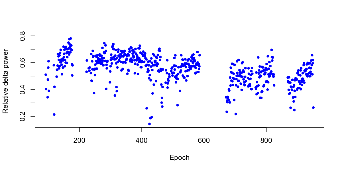
The correlation coefficient between epoch number and relative delta power is r = -0.36 and highly significant:
cor.test( delta$E ,delta$RELPSD )
    Pearson's product-moment correlation

data:  delta$E and delta$RELPSD
t = -10.304, df = 713, p-value < 2.2e-16
alternative hypothesis: true correlation is not equal to 0
95 percent confidence interval:
 -0.4221768 -0.2944507
sample estimates:
       cor
-0.3599995
Peaks/spikes
Here we review two options that perform post-processing of power
spectra derived from PSD: peaks and slope.
The peaks option gives diagnostics that indicate likely sharp
peaks in the power spectra, e.g. as caused by line noise rather than
genuine physiological oscillatory activity, which tends to produce
smoother "bumps", even though those are often called peaks in the
literature (e.g. alpha or sigma).
| Option | Example | Description |
|---|---|---|
peaks |
Perform peaks analysis | |
epoch-peaks |
Perform peaks analysis epoch-by-epoch | |
peaks-window |
7 |
Size of median filter used by peaks (default: 11 sample points) |
peaks-frq |
30,45 |
Set lower and upper bounds for the peaks analysis (default: whole spectrum) |
peaks-verbose |
Give verbose output from peaks (show smoothed spectra, etc) |
Here we take some real N2 EEG signals, and estimate the power spectra via the Welch method:
luna s.lst -o out.db
           -s ' MASK ifnot=N2 & RE & uV sig=C3
                PSD  sig=C3 max=50 spectrum dB '
We'll also look at the same signal, but with some artifact spiked in, using the SIMUL command
to introduce artificial spectral peaks (spikes) at these frequencies (i.e. as might reflect contamination from non-physiological
sources), at 5 Hz intervals from 15 Hz up to 45 Hz:
luna s.lst -o out2.db
           -s ' MASK ifnot=N2 & RE & uV sig=C3
                SIMUL frq=15,20,25,30,35,40,45 psd=500,500,500,500,500,500,500 add sig=C3
                PSD  sig=C3 max=50 spectrum dB'
add option for SIMUL adds the simulated signal onto the existing (real) C3 signal.
Plotting the resulting power spectra from both runs, we can clearly see the super-imposed artifact resulting in a more spiky or peaked spectrum:
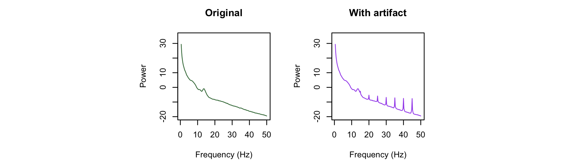
We can use the peaks option to provide one simple way of quantifying the extent of peakedness, by adding peaks to the PSD command.
By default, this would use the full spectrum to derive peak statistics: for this particular metric, it can be a good idea to avoid the lower frequenies that often contain
true bumps/peaks, e.g. resulting from oscillatory activity at those frequencies, and so we'll use the peaks-frq option instead to explicitly set the frequency range
used for the assessment of peaks: in this case 20 to 50 Hz. We'll also add the peaks-verbose option to get additional output to make the plots below. The PSD command
now reads as follows:
PSD sig=C3 max=50 spectrum dB peaks-frq=20,50 peaks-verbose '
KURT and SPK: for the original data:
destrat out.db +PSD -r CH | behead
     CH   C3
   KURT   0.317643047723098
    SPK   0.747317003553891
And for the data with spikes introduced, we see these metics are much higher:
     CH   C3
   KURT   24.053679807259
    SPK   5.39341010843361
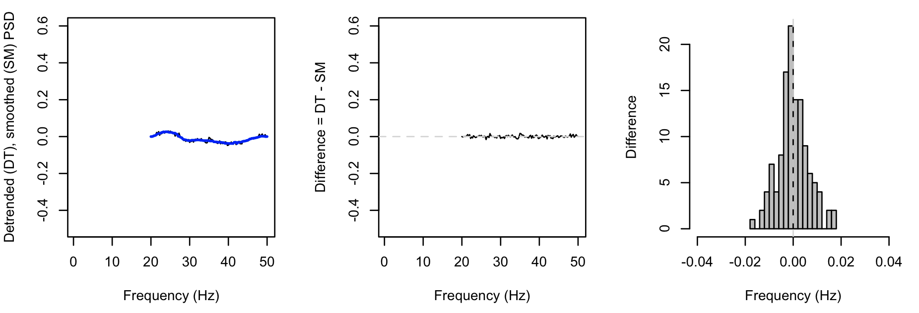
Both measures are based on the folllowing heuristic:
-
take the log-scaled power spectrum (between the frequencies specified by
peaks-frq) and scale it between 0.0 and 1.0 -
detrend this spectrum (DT: detrended spectum) and then apply a smoothing median filter (with
peaks-windowsample points) to give a smoothed spectrum (SM) -
calculate the differece (DF) between DT and SM
-
estimate the kurtosis of DF (which is the
KURTmetric) and theSPK(spikiness) as the sum of absolute values of the derivative of DF (sum( abs(diff(DF)))
The kurtosis estimate is normalized to have an expected value of 0 for
normal distributions (i.e. subtract 3.0); larger positive values
indicate greater spikiness in the spectrum. Likewise, greater values
of SPK reflect higher spikiness. The two metrics difference a
little, in that the latter is more sensitive to having many but
smaller peaks (i.e. summing over all differences), whereas the KURT
metric is more sensitive to a single, strong outlier. These metrics
do not have directly interpreted scales (e.g. they may depend on
sample rate, etc) but are designed to provide rankings across multiple
studies, to identifier outliers, with respect to the extent of spectral spikes.
Adding the peaks-verbose option gives additional output (stratified by both CH and F) that directly give the DT, SM and DF spectra
as described above: plotting these for the first instance: (black = DT, blue = SM):
Whereas, for the second instance (with the spikes introduced), we see greater values for DF (note the different x-axis for the rightmost plot, versus above):
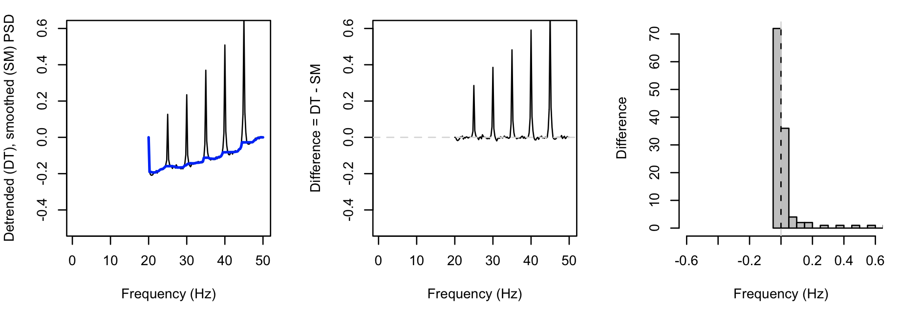
If this approach is including true bumps as outliers/spikes here,
you can try reducing peaks-window from the default of 11 (the number
of bins in the spectrum over which to do median smoothing), which
basically requires that sharper peaks by doing less smoothing.
Spectral slopes
Given a power spectrum (or multiple epoch-wise power spectra) for an individual/channel, we can estimate the spectral slope as the log-log linear regression of power on frequency. For an example of using Luna to estimate the spectral slope, see Kozhemiako et al (2021).
This is achieved by adding slope to the PSD command, and giving
the frequency interval over which the slope should be estimated. See
the references in the abovementioned pre-print to see other
applications of the spectral slope to sleep data, and justification
for looking at particular frequency ranges (i.e. in the above work,
30-45 Hz).
The other options are as follows:
| Option | Example | Description |
|---|---|---|
slope |
30,45 |
Estimate spectral slope in this frequency range |
slope-th |
2 |
Threshold to remove points when estimating slope (default: 3) |
slope-th2 |
2 |
Threshold to remove epochs when summarizing slopes over all epochs (default: 3) |
epoch-slope |
Display epoch-by-epoch slope estimates |
Luna fits the linear model of log power regressed on log frequency.
After fitting an initial model, it identifies any points (frequency
bins) that have residual values greater or less than the slope-th
threshold. This helps to avoid spikes in the power spectrum having
undue leverage on the overall slope estimate. You can also use the
peaks metrics above to flag studies that might have
issues with respect to spikes. After removing any outlier points,
Luna refits the model: the estimated slope is SPEC_SLOPE, and the
number of data points used to estimate it is in SPEC_SLOPE_N. If
looking at a 30-45 Hz (inclusive) slope with a spectral resolution of
0.25 Hz, this gives an expected 61 points; the number may be lower is
points were removed for being outliers.
Avoiding periodic acticvity that will bias spectral slope estimates
This simple implementation for estimating the spectral slope is not suitable for frequency ranges where one expects strong oscillatory activity, e.g. the sigma band during sleep, if it is to be interpreted as an index of the aperiodic component of the power spectrum. The frequency range 30-45 Hz tends to be freely of such activity and also avoids frequencies with common line noise (50/60 Hz) artifacts. As such, it is not recommended that this be used as a general method (unless other procedures have first been applied to remove oscillatory components from the signal).
Assuming multiple epochs are present in the data, Luna will also
estimate the slope epoch-by-epoch. The mean, median and the SD of these
epoch-by-epoch slopes are given in SPEC_SLOPE_MN, SPEC_SLOPE_MD
and SPEC_SLOPE_SD respectively. When combining these epoch-wise
slopes, Luna will first remove epochs that have slope estimates that
are outliers as defined by the slope-th2 (default = 3 SD).
Spectral slope outputs: (strata: CH)
| Value | Description |
|---|---|
SPEC_SLOPE |
Spectral slope of the average power spectrum |
SPEC_SLOPE_N |
Number of data points in the final model |
SPEC_SLOPE_MN |
Mean slope (over all epochs) |
SPEC_SLOPE_MD |
Median slope (over all epochs) |
SPEC_SLOPE_SD |
Slope SD (over all epochs) |
MTM
Applies the multitaper method for spectral density estimation
This provides an alternative to PSD for spectral density estimation,
that can be more efficient in some scenarios (albeit slower): the
multitaper method as described
here.
The time half bandwidth product parameter (nw) provides a way to
balance the variance and resolution of the PSD: higher values reduce
both the variance and the frequency resolution, meaning smoother but
potentially blunted and biased power spectra. The optimal choice of
nw will depend on the properties of the data and the research
question at hand. This manuscript
provides a nice review of the use of multitaper spectral analysis in the sleep
domain, along with considerations for specifying the time half
bandwidth product (nw) and the number of tapers (t). (By default,
MTM will use 2nw-1 tapers.)
As per the PSD command, the MTM command uses a concept of
segments as well as (optionally) epochs. That is, the fundamental
unit of spectral analysis is always a segment (e.g. which may be
different durations, say 4 seconds), but whether or not metrics are
summarized and output at the per-epoch (e.g. 30-second interval) level
depends on how MTM is run. Segments may often be be much smaller
than a typical epoch (e.g. 1 second) and one may wish to have highly
overlapping segments in a sliding-window style of analysis.
Running without epoch, the data is treated as a continuous signal and split into segment:
   whole recording -----------------------------|   overall stats
   |seg1|seg2|seg3|seg4|seg5|seg6|seg7|seg8|seg9|   segment-level stats (SEG)
Running with epoch, each epoch is split into segments; at least one epoch must fit in each segment:
   whole recording -----------------------------|   overall stats
   | epoch1 ------| epoch2-------| epoch3 ------|   epoch-level stats (E)
   |seg1|seg2|seg3|seg1|seg2|seg3|seg1|seg2|seg3|   segment-level stats (SEG)
Analyses can be performed epoch-wise, but without verbose epoch-level
output being emitted: in this case, one just uses the epoch flag.
To get epoch-level outputs, use epoch-output; to get full spectra
(i.e. stratified by F) output, also add epoch-spectra. Parallel
options exist to control the level of segment-wise outputs
(segment-output and segment-strata). Note that, depending on the
dataset and other parameters, the outputs from segment-strata (or
epoch-strata) could be very large: using text-table outputs is
advisable in this scenario.
As well as core spectral power metrics (either summed by frequency band, or per bin), this command calculates a number of other values based on the spectral analysis:
-
ratios between different band powers
-
so-called spectral skew, kurtosis and CV (coefficient of variation) based on the distribution of segments (within each epoch)
Parameters
| Parameter | Example | Description |
|---|---|---|
sig |
C3,C4 |
Which signals to analyse |
epoch |
Report epoch-level results | |
nw |
4 |
Time half bandwidth product (default 3, typically: 2, 5/2, 3, 7/2, or 4) |
t |
7 |
Number of tapers (default 2*nw-1, i.e. 5) |
segment-sec |
30 | Segment size (default 30 seconds) |
segment-inc |
30 | Segment increment/step (default 30 seconds) |
min |
0.5 |
Maximum frequency for power spectra (default is 20Hz) |
max |
25 |
Maximum frequency for power spectra (default is 20Hz) |
dB |
Report power in dB units |
Output control
| Parameter | Description |
|---|---|
epoch-output |
Run in epoch mode and output epoch-wise statsistics (except the full spectra) |
epoch-strata |
If running in epoch mode, output full per-epoch power spectra |
segment-output |
Output per-segment statistics (except the full spectra) |
segment-spectra |
Output per-segment full power spectra |
dump-tapers |
Report the taper coefficients in the output |
add |
Add new channels with MTM power values, in format mtm_CH_F |
Misc analysis parameters
| Parameter | Example | Description |
|---|---|---|
speckurt |
Report epoch-level kurtosis per band | |
speckurt3 |
Use unadjusted kurtosis vales, i.e. N(0,3) has expected kurtosis of 3.0, not 0 | |
ratio |
DELTA/ALPHA,DELTA/BETA |
Output band power ratios, e.g. delta/alpha and delta/beta |
ratio1 |
Compute raw power ratios as a/(1+b) | |
mean-center |
Mean center segments prior to analysis |
Spectral slope parameters
| Parameter | Example | Description |
|---|---|---|
slope |
Output the spectral slope | |
epoch-slope |
Output the spectral slope per epoch (or slope-epoch) |
|
slope-th |
4 | SD threshold at which to remove individual power estimates (default: 3 ) |
slope-th2 |
4 | SD threshold at which to remove epochs (default: 3 ) |
Output
Whole-signal power spectra (strata: CH x F)
| Variable | Description |
|---|---|
MTM |
Absolute spectral power via the multitaper method |
MTM_MD |
With epoch, median power over epochs |
MTM_SD |
With epoch, SD of power over epochs |
Whole-signal band power (strata: CH x B)
| Variable | Description |
|---|---|
MTM |
Absolute spectral band power via the multitaper method |
MTM_MD |
With epoch, median power over epochs |
MTM_SD |
With epoch, SD of power over epochs |
REL |
Relative spectral band power via the multitaper method (denom = total power) |
REL_MD |
With epoch, median relative power over epochs |
REL_SD |
With epoch, SD of relative power over epochs |
Ratios of band power (option: ratio; strata: CH x B1 x B1)
| Variable | Description |
|---|---|
RATIO |
Ratio (or mean ratio over epochs, if epoch) |
RATIO_MD |
With epoch, median ratio over epochs |
RATIO_SD |
With epoch, SD of ratios over epochs |
Epoch-level power spectra (option: epoch, strata: E x CH x F)
| Variable | Description |
|---|---|
MTM |
Spectral power via the multitaper method |
Epoch-level band power (option: epoch, strata: E x CH x B)
| Variable | Description |
|---|---|
MTM |
Spectral power via the multitaper method |
REL |
Relative spectral power via the multitaper method |
Epoch-wise segment-level band power (option: epoch, segment-output; strata: CH x E x SEG x B)
| Variable | Description |
|---|---|
MTM |
Spectral power via the multitaper method |
REL |
Relative spectral power via the multitaper method |
Segment-level output (option: segment-output; strata: CH x SEG)
| Variable | Description |
|---|---|
START |
Start of segment (seconds) |
STOP |
End of segment (seconds) |
DISC |
Flag (0/1) indicating if a segment spans a discontinuity |
Epoch-wise segment-level output (option: epoch, segment-output; strata: CH x E x SEG)
| Variable | Description |
|---|---|
START |
Start of segment (seconds) |
STOP |
End of segment (seconds) |
DISC |
Flag (0/1) indicating if a segment spans a discontinuity |
Epoch-level ratios of band power (options: ratio, epoch-output; strata: CH x B1 x B1)
| Variable | Description |
|---|---|
RATIO |
Ratio (or mean ratio over epochs, if epoch) |
RATIO_MD |
With epoch, median ratio over epochs |
RATIO_SD |
With epoch, SD of ratios over epochs |
Alternate statistcs (spectral skew, kurtosis and CV)
Band-wise statistics (option: speckurt; strata: CH x B)
| Variable | Description |
|---|---|
SPECCV |
CV of spectral band power |
SPECSKEW |
Skewness of spectral band power |
SPECKURT |
Kurtosis of spectral band power |
The above three metrics are also defined:
- per epoch per channel per epoch (stata:
ExCHxB) - averaged over channels per epoch (strata:
ExB) - when using
speckurt3
Adding channels
If the add option is specified, multiple new channels will be added
with the computed power values (same sample rate as the original
signal, with values averaged over any overlapping windows). If adding
channels, it is typically a good idea to reduce the number of
frequency bins considered (with min and max) as one channel is
added per bin/channel.
Example
To compare results for the N2 power spectra up to 20 Hz, from PSD and MTM
for the three tutorial individuals:
luna s.lst -o out.db -s ' MASK ifnot=N2 & RE
            & PSD sig=EEG dB spectrum max=20
            & MTM sig=EEG dB tw=15 max=20'
This gives some output describing the properties of the MT analysis in the console:
 CMD #4: MTM
   options: dB=T max=20 sig=EEG tw=15
  assuming all channels have the same sample rate of 125Hz:
    time half-bandwidth (nw) = 15
    number of tapers         = 29
    spectral resolution      = 1Hz
    segment duration         = 30s
    segment step             = 30s
    FFT size                 = 4096
    number of segments       = 375
    adjustment               = none
  processed channel(s): EEG
Using library(luna) in R to view the resulting output:
k <- ldb( "out.db" )
mtm <- lx( k , "MTM" , "CH" , "F" )
psd <- lx( k , "PSD" , "CH" , "F" )
par(mfcol=c(1,3))
yr <- range( c( mtm$MTM , psd$PSD ) )
for (i in unique( mtm$ID ) ) {
plot( mtm$F[mtm$ID==i] ,  mtm$MTM[mtm$ID==i] , type="l" , col="purple" , lwd=2 , xlab="Frequency (Hz)" , ylab="Power (dB)" , ylim=yr )
lines( psd$F[psd$ID==i] , psd$PSD[psd$ID==i] , type="l" , col="orange" , lwd=2 )
legend(12,20,c("MTM","PSD"),fill=c("purple","orange"))
}
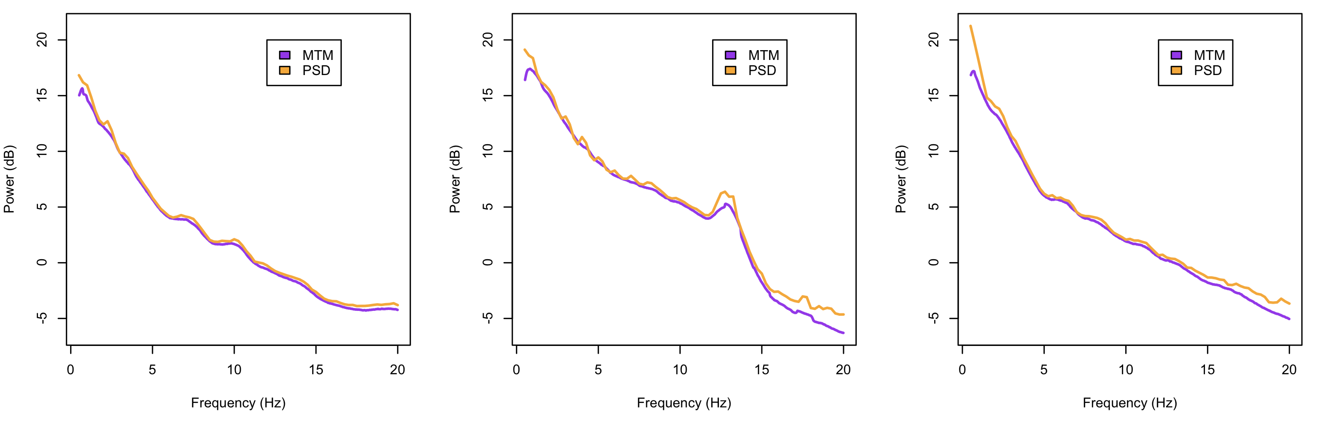
As expected, in this particular scenario and with long signals, both methods produce similar results.
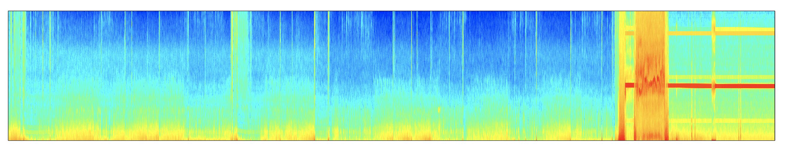
As a second example, here is a whole-night MT spectrogram, performed within lunaR:
library(luna)
lattach( lsl( "s.lst" ) , 1 )
k <- leval( "MTM sig=EEG tw=15 max=30 epoch dB" )
Examing the output:
lx(k)
MTM : CH_F CH_F_SEG
And plotting a heatmap:
d <- k$MTM$CH_F_SEG
lheatmap( d$SEG , d$F , d$MTM )
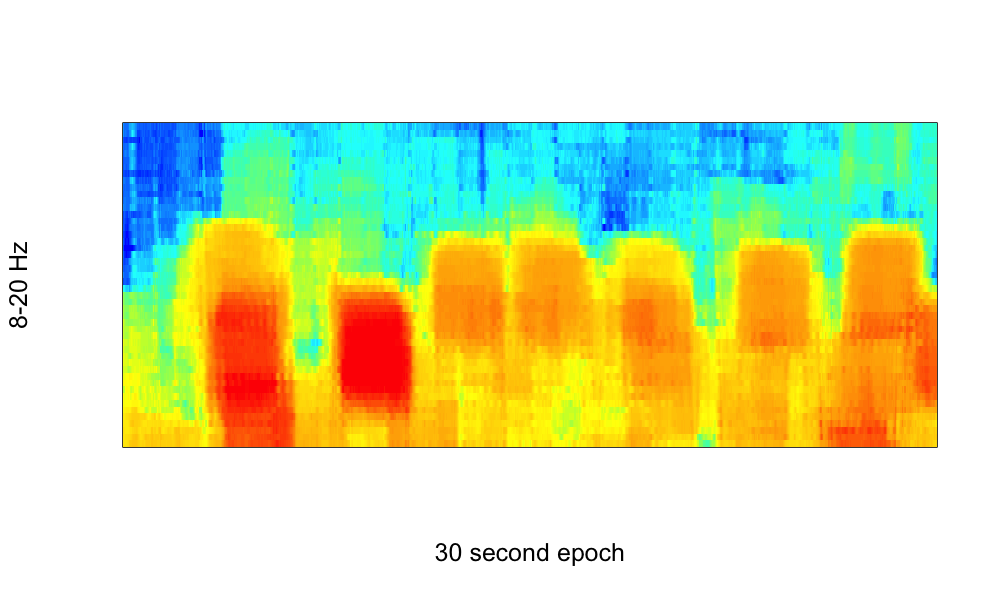
As a third example: here is an application of MTM on a smaller segment of data (a single epoch), which shows sleep spindles in the MTM spectrogram (plotting the results in the range of 8 to 20 Hz), generated by the commands:
MTM segment-sec=2.5 segment-inc=0.02 epoch nw=5 max=30 dB
Note the use of a small (2.5 seconds) segment size, which is shifted only 0.02 seconds at a time, and so gives a considerable smoothing of estimates in the time domain (which may or may not be desirable, depending on the goal of the analysis.)
FFT
Applies the basic discrete Fourier transform to a signal
In contrast to Welch (PSD) or multi-taper (MTM)
approaches, the FFT performs that same function (for a single, real,
1-dimensional signal) as the fft() function in R or Matlab, i.e.
the DFT with no windowing or tapering, and which will have as many
points as there are samples. As such, this is intended for use with
simple/short signals, where one wants this exact quantity, e.g. if
validating a computation, as we did here. For real
data (especially long, whole night recordings), PSD and MTM will
provide better estimates of the power spectrum.
Info
Practically, for very long signals, FFT will return a very large/dense spectrum, which
might make the destrat output mechanism struggle; if you really want this, run with the -t command-line option
to produce text table outputs.
Parameters
| Parameter | Example | Description |
|---|---|---|
sig |
C3,C4 |
Which signal(s) to analyse |
verbose |
Output additional variables (see below) |
Output
Whole-signal power spectra (strata: CH x F)
| Variable | Description |
|---|---|
PSD |
Raw power spectral density |
DB |
10log10(PSD) |
Optional output (option: verbose, strata: CH x F)
| Variable | Description |
|---|---|
RE |
Real part of the DFT |
IM |
Imaginary part of the DFT |
UNNORM_AMP |
Unnormalized amplitude |
NORM_AMP |
Normalized amplitude |
Examples
This command is a wrapper around the same FFT/DFT analysis performed by the fft command line function:
luna -d fft 100 < data.txt
See this vignette for a description of the outputs, and an example of usage (i.e. here, the
only difference is that FFT command operates on EDF channels, whereas the example above is based on reading a text file.)
IRASA
Implements the Irregular-Resampling Auto-Spectral Analysis method
Implements the IRASA method as described here, which seeks to partition power spectra into periodic (oscillatory) and aperiodic (fractal) components.
Parameters
| Parameter | Example | Description |
|---|---|---|
sig |
C3,C4 |
Which signal(s) to analyse |
h-min |
1.05 | Minimum resampling factor (default 1.05) |
h-max |
1.95 | Maximum resampling factor (default 1.95) |
h-steps |
19 | Number of steps between h-min and h-max (default 19, i.e. 0.05 increments) |
dB |
Report log-scaled power | |
epoch |
Report epoch-level statistics | |
min |
1 | Minimum frequency to include in the output (default 1 Hz) |
max |
30 | Maximum frequency to include in the output (default 30 Hz) |
Secondary parameters
| Parameter | Example | Description |
|---|---|---|
segment-mean |
Use the mean (rather than median) across segments, within epoch | |
epoch-mean |
Use the mean (rather than median) across epochs | |
fast |
Use a faster (but less accurate) linear resampling method | |
segment-sec |
5 | Set the Welch segment size (default 4 seconds) |
segment-overlap |
2.5 | Set the Welch segment overlap/increment (default 2 seconds) |
no-window |
No windowing for Welch method | |
hann |
Use a Hann window for Welch method | |
hamming |
Use a Hamming window for Welch method | |
tukey50 |
Use a Tukey window for Welch method |
Output
Whole-signal power spectra (strata: CH x F)
| Variable | Description |
|---|---|
LOGF |
Log-scaled frequency F (if dB specified) |
APER |
Aperiodic component of the power spectrum |
PER |
Periodic component of the power spectrum |
Whole-signal slope statistics (strata: CH)
| Variable | Description |
|---|---|
SPEC_SLOPE |
Spectral slope (based on aperiodic component) |
SPEC_INTERCEPT |
Spectral intercept (based on aperiodic component) |
SPEC_RSQ |
R-sq for above fit |
SPEC_SLOPE_N |
Number of non-outlier data points in slope estimate |
Optional epoch-level output (option: epoch, strata: E x CH x F)
| Variable | Description |
|---|---|
LOGF |
Log-scaled frequency F ( if dB specified) |
APER |
Aperiodic component of the power spectrum |
PER |
Periodic component of the power spectrum |
Epoch-level slope statistics (option: epoch, strata: E x CH)
| Variable | Description |
|---|---|
SPEC_SLOPE |
Epoch spectral slope (based on aperiodic component) |
SPEC_INTERCEPT |
Epoch spectral intercept (based on aperiodic component) |
SPEC_RSQ |
Epoch R-sq for above fit |
SPEC_SLOPE_N |
Epoch number of non-outlier data points in slope estimate |
Examples
We use Luna's SIMUL command to generate random time series
data, specifying a 1/f^alpha slope with alpha set to 2, as well as a periodic
component centered at 15 Hz. We generate 3000 seconds of data, with a sample
rate of 256 Hz:
luna . -o out.db --nr=3000 --rs=1 \
       -s ' SIMUL alpha=2 intercept=1 frq=15 psd=10 w=0.1 sig=S1 sr=256
            PSD sig=S1 spectrum max=30 slope=1,30 dB
            IRASA sig=S1 dB h-max=4'
S1 using first PSD (Welch method)
and then IRASA. For PSD, we have to explicitly request that the spectral slope be estimated (slope=1,30)
which indicates a log-log regression of power on frequency (after removing outlier points). We expect this
estimate of slope to be biased by the oscillatory peak at 15 Hz. In contrast, IRASA will generate
two spectra, the aperiodic and periodic components, and estimate the slope (using the same approach as PSD)
only on the aperiodic component.
To compare like-with-like, we use a range of 1 to 30 Hz in both cases
(this is the default for IRASA). We set the resampling factor h to
have a maximum value of 4, which implies an evaluated range of 1/4 =
0.25 Hz to 30 * 4 = 120 Hz.
  specified frequency range is 1 - 30 Hz
  full evaluated frequency range given h_max = 4 is 0.25 - 120 Hz
Extracting the estimated slopes from both methods: Welch estimates are a little biased (-1.9 instead of -2, i.e. minus alpha) and has a modest model fit (R-sq ~50%):
destrat out.db +PSD -r CH | behead
                 SPEC_RSQ   0.50951
               SPEC_SLOPE   -1.91503
destrat out.db +IRASA -r CH | behead
                 SPEC_RSQ   0.99874
               SPEC_SLOPE   -2.03858
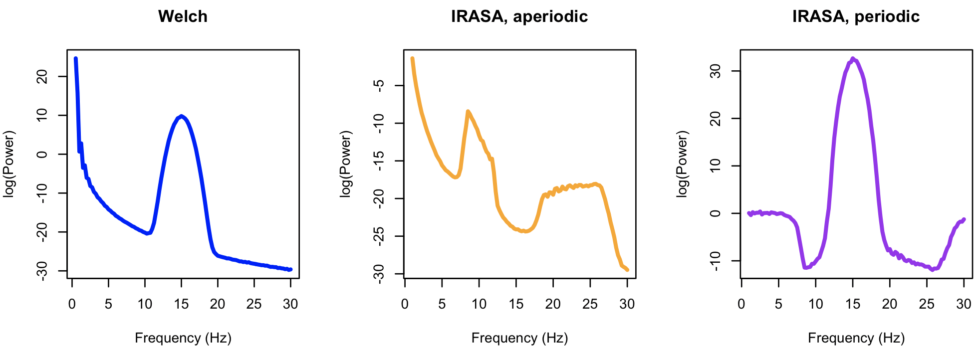
We can visualize the three resulting power spectra as follows, in R:
k <- ldb( "out.db" )
par(mfcol=c(1,3))
d <- k$PSD$CH_F
plot( d$F, d$PSD, type="l", lwd=3, col="blue", xlab="Frequency (Hz)", ylab="log(Power)", main="Welch" )
i <- k$IRASA$CH_F
plot( i$F, i$APER, type="l", lwd=3, col="orange", xlab="Frequency (Hz)", ylab="log(Power)", main = "IRASA, aperiodic" )
plot( i$F, i$PER, type="l", lwd=3, col="purple", xlab="Frequency (Hz)", ylab="log(Power)", main="IRASA, periodic" )
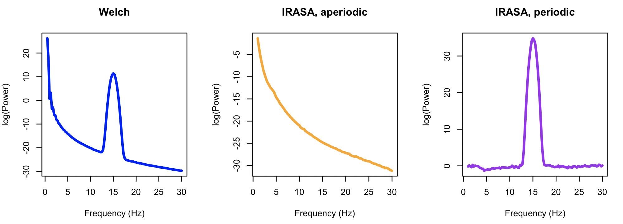
As nicely illustrated by Gerster et al. (2021), IRASA
is not infallible - for instance, if there are very broad oscillatory peaks and the maximum resampling
factor is not sufficiently high, it can fail to properly separate out aperiodic and periodic components
(see their Figure 6). We can recapitulate this property by increasing the peak width (w in SIMUL)
and reduced the resampling factor (h-max in IRASA):
luna . -o out.db --nr=3000 --rs=1 \
       -s ' SIMUL alpha=2 intercept=1 frq=15 psd=10 w=1 sig=S1 sr=256
            PSD sig=S1 spectrum max=30 slope=1,30 dB
            IRASA sig=S1 dB h-max=2'
This is of course an extreme example (i.e. with a very large amplitude, broad oscillatory peak), but nonetheless shows one failure mode of IRASA. In practice, examining the shape of the aperiodic spectrum (i.e. which should be approximately striaght on a log-log or semi-log plot) will indicate if resulting slope estimates are likely biased by oscillatory activity.
HILBERT
Applies filter-Hilbert transform to a signal, to estimate envelope and instantaneous phase
This function can be used to generate the envelope of a (band-pass filtered) signal.
Parameters
| Parameter | Example | Description |
|---|---|---|
sig |
sig=EEG |
Which signal(s) to apply the filter-Hilbert to |
f |
f=0.5,4 |
Lower and upper transition frequencies |
ripple |
ripple=0.02 |
Ripple (0-1) |
tw |
tw=0.5 |
Transition width (in Hz) |
tag |
tag=v1 |
Additional tag to be added to the new signal |
phase |
phase |
Generate a second new signal with instantaneous phase |
Outputs
No formal output, other than one or two new signals in the in-memory
representation of the EDF, with _hilbert_mag and (optionally)
_hilbert_phase suffixes.
Example
Using lunaR, with nsrr02 attached, we will use the filter-Hilbert method to
get the envelope of a sigma-filtered EEG signal. After attaching the sample, we then drop all signals
except the one of interest:
leval( "SIGNALS keep=EEG" )
We then apply the filter-Hilbert method, which will generate two new
channels, EEG_hilbert_11_15_mag and EEG_hilbert_11_15_phase:
leval( "HILBERT sig=EEG f=11,15 ripple=0.02 tw=0.5 phase" )
For illustration, we'll also generate a copy of the original signal:
leval( "COPY sig=EEG tag=SIGMA" )
and then apply a bandpass filter to it, in the same sigma range as above:
leval( "FILTER sig=EEG_SIGMA bandpass=11,15 ripple=0.02 tw=0.5" )
Note
Unlike HILBERT, FILTER modifies the source channel,
which is why we COPY-ed the original channel first.
We now have four signals in the in-memory representation of the EDF:
lchs()
[1] "EEG"                     "EEG_hilbert_11_15_mag"
[3] "EEG_hilbert_11_15_phase" "EEG_SIGMA"
To view some of the results, we can use ldata() to extract signals
for a particular epoch. For better visualization, here we'll select
smaller (15 second) epochs:
lepoch(15)
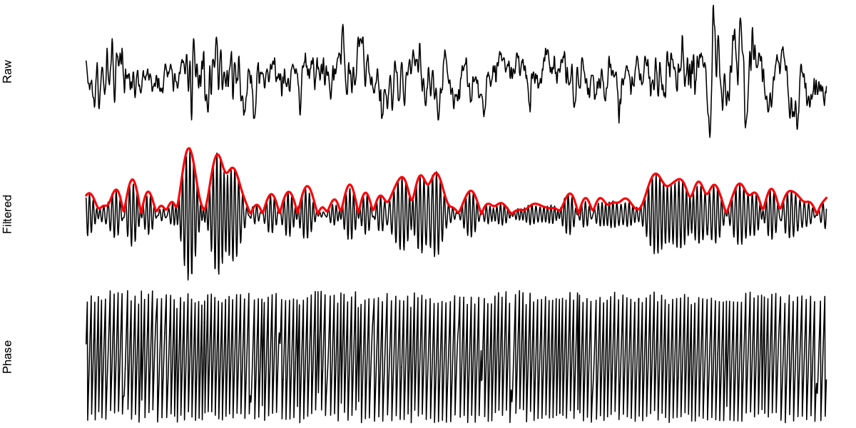
We can then pull all four signals for given (set of) epoch(s), say number 480:
d <- ldata( 480 , chs=lchs() )
par(mfcol=c(3,1),mar=c(0,4,0,0),xaxt='n',yaxt='n')
plot( d$SEC , d$EEG , ylab = "Raw" , type="l" ,axes=F)
plot( d$SEC , d$EEG_SIGMA , ylab = "Filtered" , type="l" , axes=F)
lines( d$SEC , d$EEG_hilbert_11_15_mag , col="red" , lwd=2 )
plot( d$SEC , d$EEG_hilbert_11_15_phase , ylab = "Phase" , type="l" , axes=F)
CWT
Applies a continuous wavelet transform by convolution with a complex Morlet wavelet
The CWT is the basis of the SPINDLE
command. This command allows you to generate new signals in the EDF
that correspond to the underlying CWT, e.g. for plotting, or getting
insight into the performance of SPINDLES under different
circumstances.
Parameters
| Parameter | Example | Description |
|---|---|---|
sig |
sig=EEG |
Which signal(s) to apply the CWT to |
fc |
fc=15 |
Wavelet center frequency |
cycles |
cycles=12 |
Bandwidth of the wavelet, specified in terms of the number of cycles |
tag |
tag=v1 |
Additional tag to be added to the new signal |
phase |
phase |
Generate a second new signal with wavelet's phase |
Outputs
No formal output, other than one (or two) new signals appended to the in-memory representation of the EDF.
CWT-DESIGN
Display the properties of a complex Morlet wavelet transform
This command does not operate on EDFs per se; rather, it produces analytic output on the properties of a continuous wavelet transform (CWT) given the design parameters.
Wavelet bandwidth can be specifed in one of two ways: by giving the
number of cycles (cycles option) OR by specifying the time-domain
full width at half maximum (FWHM) value (in seconds). See this
manuscript
for a discussion of the advantages of this latter specificiation.
In both cases, the CWT-DESIGN will estimate the implied FWHM in the frequency domain,
i.e. the tightness of the wavelet around the specified central frequency (fc).
Parameters
| Parameter | Example | Description |
|---|---|---|
fs |
fs=200 |
Sample rate |
fc |
fc=15 |
Center frequency |
fwhm |
fwhm=1 |
Time-domain FWHM (use instead of cycles) |
cycles |
cycles=7 |
Number of cycles in wavelet (use instead of fwhm) |
Outputs
Time/frequency domain FWHM (strata: PARAM)
| Variable | Description |
|---|---|
FWHM |
Specified time-domain full width at half max (if fwhm option given) (secs) |
FWHM_F |
Estimated frequency-domain FWHM (Hz) |
FWHM_LWR |
Estimated lower half-max frequency bound (Hz) |
FWHM_UPR |
Estimated upper half-max frequency bound (Hz) |
Frequency response for wavelet (strata: PARAM x F)
| Variable | Description |
|---|---|
MAG |
Magnitude of response (arbitrary units) |
Wavelet coefficients (strata: PARAM x SEC)
| Variable | Description |
|---|---|
REAL |
Real part of wavelet |
IMAG |
Imaginary part of wavelet |
Example
To display the properties of a wavelet with center frequency of 15 hz and 12 cycles, applied to a signal with sample rate of 12 Hz.
luna s.lst 1 -o out.db -s 'CWT-DESIGN fc=15 cycles=12 fs=200'
Note
The default value of cycles for the SPINDLES command is 7 cycles.
Equivalently, without an EDF/sample list, you can use the --cwt
parameter and pipe the parameters (fc, cycles and fs). Here we
use it for both 11 Hz and 15 Hz wavelets. Also, note the use of
-a instead of -o for the second command, so that the output of the
second command appends (rather than overwrites) the existing
out.db:
echo "fc=11 cycles=12 fs=200" | luna --cwt -o out.db
echo "fc=15 cycles=12 fs=200" | luna --cwt -a out.db
Using lunaR to view the output:
k <- ldb("out.db")
lx(k)
CWT_DESIGN : PARAM F_PARAM PARAM_SEC
PARAM (a description of the input parameters) and F (frequency):
d <- lx( k , "CWT_DESIGN" , "PARAM" , "F" )
plot( d$F[ d$PARAM == "11_12_200" ]  , d$MAG[ d$PARAM == "11_12_200" ] ,
 xlim=c(0,20) , type="l" , lwd=2 , col="blue" ,
 xlab="Frequency (Hz)" , ylab="Amplitude" , ylim=c(0,1) )

lines( d$F[ d$PARAM == "15_12_200" ]  , d$MAG[ d$PARAM == "15_12_200" ] ,
 lwd=2 , col="red" )

legend( 2 , 0.9 , c("11 Hz","15 Hz") , fill = c("blue","red") )
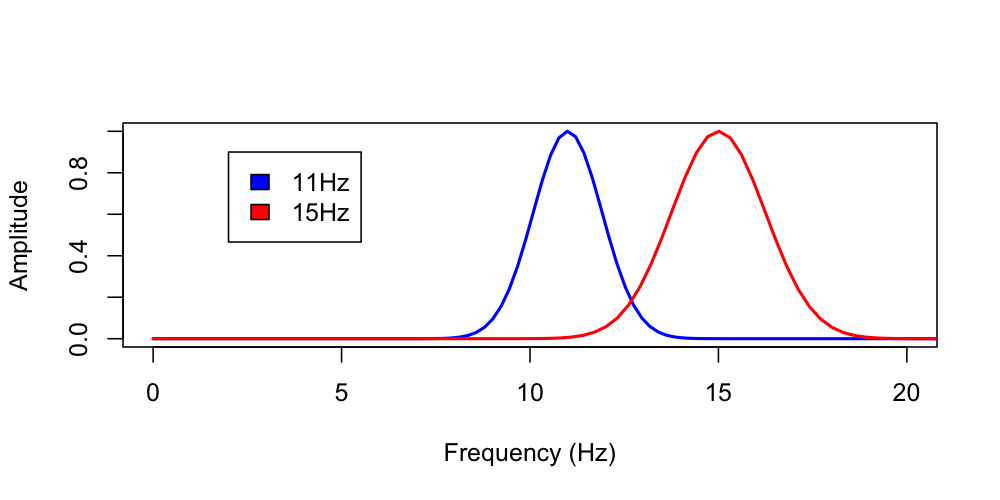
Looking at the estimated frequency domain FWHM values, we see these correspond to the y=0.5 (i.e. 50%) values for each wavelet, at lower and upper valeus respectively.
lx( k , "CWT_DESIGN" , "PARAM" )
ID      PARAM    FWHM_F  FWHM_LWR  FWHM_UPR
.   11_12_200  2.197802   9.89011  12.08791
.   15_12_200  3.003003  13.51351  16.51652
PCOUPL
Generic phase/event coupling analysis
This command implements that same functions used by
SPINDLES when evaluating spindle/SO phase
coupling and overlap. Here, the functionality has been extracted out of the
context of the SPINDLES command, to make it generically useful. That is, given a set of annotations
and one or more signals, this will:
-
apply the filter-Hilbert method to determine instantaneous phase of the signal
-
given a defined anchor for annotation events (e.g. start, middle or end) it assess whether or not the events occur randomly with respect to the phase of the signal, using randomization to generate surrogate time series
For the purpose of calculating overlap statistics, phase bins are fixed in 18 20-degree bins.
Parameters
| Option | Example | Description |
|---|---|---|
sig |
C3 |
One or more signals (for determining phase) |
events |
arousal |
One or more annotation classes |
lwr |
3 | Lower frequency for filter-Hilbert |
upr |
8 | Upper frequency for filter-Hilbert |
anchor |
start |
Anchor for events (start, middle/mid or stop/end) |
nreps |
1000 | Number of permutations |
Secondary parameters
| Option | Example | Description |
|---|---|---|
tw |
0.5 | Transition width for Kaiser window FIR |
ripple |
0.01 | Ripple parameter for Kaiser window FIR |
perm-whole-trace |
Permute signals across whole recording (not within epoch) | |
fixed-epoch-dur |
20 | If using generic epochs, set a fixed epoch size for permutation |
Note: cannot run within-epoch permutation with generic epochs: add fixed-epoch-dur or perm-whole-trace
Outputs
Phase coupling statistics (strata: ANNOT x CH)
| Variable | Description |
|---|---|
ANGLE |
Mean phase angle (degrees) |
MAG |
Coupling magnitude (observed statistic) |
MAG_Z |
Permutation-basewd Z-score for coupling magnitude |
MAG_NULL |
Mean coupling statistic under the null |
MAG_EMP |
Empirical p-value |
PV |
Asymptotic p-value |
SIGPV_NULL |
Proportion of asymptotic p<0.05 under the null |
N |
Number of events |
Phase-bin overlap statistics (strata: ANNOT x CH x PHASE)
| Variable | Description |
|---|---|
OVERLAP |
Observed count of event anchors per signal phase bin |
OVERLAP_EXP |
Expected count based on permutations |
OVERLAP_EMP |
Empirical p-value based on permutations |
OVERLAP_Z |
Z-score based on permutations |
Example
Here we use SPINDLES to assess spindle/SO coupling:
luna s.lst 2 -o out.db \
  -s ' MASK ifnot=N2 & RE
       SPINDLES sig=EEG annot=SP nreps=1000 so mag=2
       WRITE-ANNOTS annot=SP file=sp.annot '
Looking at some of the relevant outputs: here we see a mean phase angle of 260 degrees (i.e. rising slope of the SO, just before the peak at 270 degrees), and an indication that there is significantly non-random coupling (i.e. high Z score, etc):
destrat out.db +SPINDLES -r F CH -v COUPL_ALL_MAG COUPL_ALL_MAG_Z COUPL_ALL_PV COUPL_ALL_ANGLE N | behead
    COUPL_ALL_ANGLE   260.205
      COUPL_ALL_MAG   0.24571
    COUPL_ALL_MAG_Z   5.94923
       COUPL_ALL_PV   1.82e-14
                  N   524
(Note the COUPL_ALL statistics are based on all spindles, not just
those that overlap a detected SO; we focus on this, as this will be
more comparable with the application of PCOUPL below.)
Now, imagine instead that we'd used another method to determine
spindles, outside of Luna. Or, indeed, that "spindles" here may
instead reflect any type of event, e.g. arousals, apnea, etc (and
instead of the EEG, the sig here could be any type of rhythmic
signal, e.g. airflow, etc). Here we can use PCOUPL to
(approximately - see below) recapitulate the internals of SPINDLES (again, noting
that PCOUPL can be used generically). We attach the previous spindle calls with annot-file,
and then specify these with events:
luna s.lst -o out.db \
     annot-file=sp.annot \
   -s ' MASK ifnot=N2 & RE
        PCOUPL sig=EEG lwr=0.5 upr=4 nreps=1000 events=SP anchor=mid '
Here we use the mid-point of the spindle (anchor=mid) to assign phases to events. The console log
tells us that (as above) the 524 spindle events have been mapped to a non-masked (i.e. N2) portion of
the recording:
 CMD #3: PCOUPL
   options: anchor=mid events=SP lwr=0.5 nreps=1000 ripple=0.01 sig=EEG tw=0.5 upr=4
  using epoch duration of 30s for within-epoch shuffling
  processing EEG
  done filter-Hilbert...
   - processing SP
  mapped 524 of 524 events
Looking at the primary outputs we see (broadly) similar results as above:
destrat out.db +PCOUPL -r ANNOT CH | behead
        ANNOT   SP
           CH   EEG
        ANGLE   277.451
          MAG   0.1665
      MAG_EMP   0.0159
     MAG_NULL   0.0495
        MAG_Z   3.8659
            N   524
           PV   4.8e-07
   SIGPV_NULL   0.162
That is, both asymptotic (PV) and empirical (MAG_EMP) p-values are significant, and the mean angle is near 270 degrees.
Why aren't these identical to the above (given that SPINDLES also uses
a filter-Hilbert band of 0.5 - 4 Hz by default)? This primarily
relates to the anchor used. Internally, SPINDLES actually uses the
point of maximal wavelet coefficient as the "anchor". In this (more
generic) function, there may not be an equivalent, and so PCOUPL
will use either the start, mid-point or end (i.e. based only on the start/stop times of the spindle).
This slightly changes the mean angle and also reduces the magnitude of phase coupling a
small amount. So, for spindle/SO analysis it would still be
preferrable to use SPINDLES, but for other types of (more generic)
phase-coupling analysis, PCOUPL would be appropriate.
Finally, we can also pull out the count of events per 20-degree bin of the slow phase (excluding some columns from the output for clarity):
destrat out.db +PCOUPL -r ANNOT CH PHASE
PHASE   OVERLAP OVERLAP_EXP OVERLAP_EMP   OVERLAP_Z
10      20      28.537      0.95304      -1.5539
30      28      28.7        0.57742      -0.1249
50      16      28.432      0.99800      -2.2381
70      25      27.921      0.75124      -0.5687
90      22      27.395      0.86013      -1.0074
110     20      27.798      0.93706      -1.3992
130     21      27.981      0.94005      -1.3821
150     25      28.403      0.76323      -0.6399
170     29      29.087      0.52047      -0.0157
190     32      29.782      0.35164       0.4230
210     29      30.542      0.62137      -0.2728
230     24      30.152      0.88111      -1.0892
250     39      30.688      0.08191       1.5959
270     37      30.257      0.12987       1.2361
290     47      29.859      0.00099       3.2154
310     46      29.721      0.00599       2.9167
330     33      29.42       0.26473       0.6731
350     31      29.325      0.39560       0.3096
That is, for bins 290 (280-300) and 310 (300-320) we see more events
than (OVERLAP) than we'd expect by chance (OVELAP_EXP), leading to positive
Z scores and significant (1-sided) empirical p-values.
EMD
Empirical mode decomposition
Empirical mode decomposition, or the Hilbert-Huang transform (described here). Currently, EMD is applied to the entire duration of the recording (i.e. it does not work epoch-wise).
Parameters
| Option | Example | Description |
|---|---|---|
sig |
C3 |
Specify the channels to which EMD will be applied |
tag |
EMD |
Change the default _IMF_N tag, e.g. C3_IMF_1 to C3_EMD_1 |
sift |
20 | Maximum number of sifting iterations (default: 20) |
imf |
10 | Number of intrinsic mode functions to extract (default: 10) |
Outputs
There is no formal output from the EMD command, other than generating new channels
that are added to the in-memory EDF. That is, the intrinsic mode functions (up to imf of them) are
written to the EDF as new channels (with the same sample
rate as the original signal) and given suffixes _IMF_1, _IMF_2,
etc. The residual component is given the suffix _IMF_0.
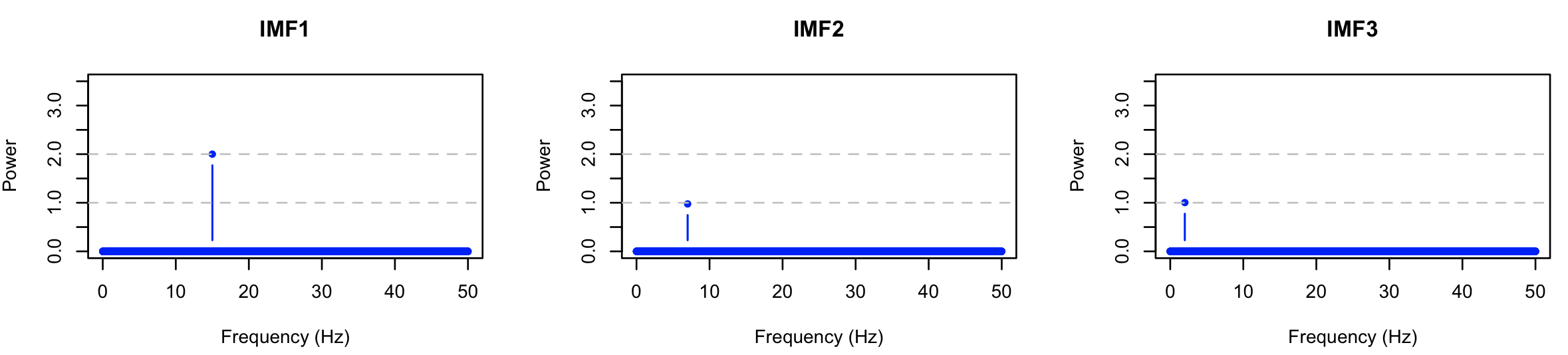
Example
Here we use the SIMUL command to generate 5
minutes of a simple, stationary signal, that comprises three
independent sine-waves, at 2, 7 and 15 Hz, with power of 1, 1 and 2
units, respectively.
luna . --nr=300 --rs=1 -o out.db \
       -s ' SIMUL frq=2,7,15 psd=1,1,2 sig=S1 sr=100
            EMD sig=S1 imf=3
            FFT
            MATRIX file=s1.txt'
The EMD command by default takes requires the channel(s) (sig) to be
specified. In this example, because we know there are only three
components, we set imf to 3 (the default is to return 10
components). Note that the first three components will be identical
whether or not imf is specified, as this option only impacts what
is output (and the residual component).
The FFT command performs a
DFT, for the original signal S1 but also the new
signals attached by EMD: namely, S1_IMF_1, S1_IMF_2 and
S1_IMF_3. Finally, the MATRIX command dumps the raw signals to a
file s1.txt (for plotting).
After running the above, we can first look at the raw signals (in s1.txt), for the original simulated signal S1 (here
showing just two seconds of the recording):

and likewise for the three components extracted by EMD:
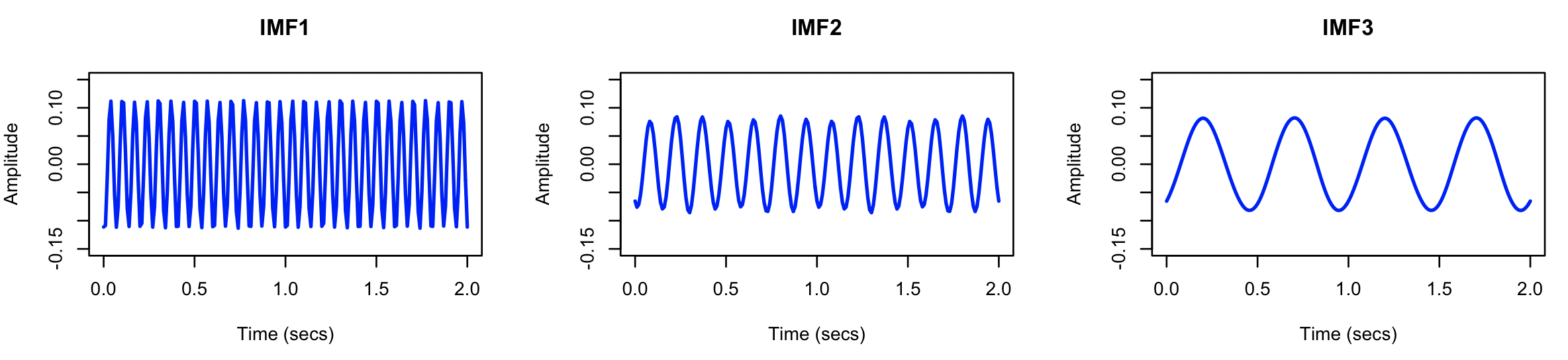
It does indeed look as though EMD has extracted three sine waves,
with the first being the fastest (as expected given the sifting/EMD
algorithm) and also of greater amplitude (as expected given the
simulation).
We can look at the spectral properties of the original signal and the EMD-derived components. As expected, the original signal has power at exactly 2, 7 and 15 Hz (in a ratio of 1:1:2):

Performing the FFT separately on each component, we see that EMD has in this instance successfully isolated the three simulated components:
Note
In practice, although EMD can be more appropriate for working with nonlinear and nonstationary signals compared to other time/frequency decomposition methods, there can still be issues, e.g. arising from boundary effects or highly variably signals, as discussed here. Simply put, like most things, EMD is not guaranteed to magically work as expected every time...
MSE
Calculates per-epoch multi-scale entropy statistics
This function estimates multi-scale entropy (MSE) as described in the approach of Costa et al, which is based on the concept of sample entropy.
In short, there are two steps: first, the time series is
coarse-grained, dependent on scale parameter s (typically varied
between 1 and 20); second, sample entropy is calculated for each
coarse-grained time series, dependent on parameters m and r.
Parameters m and r define the pattern length and the similarity
criterion respectively, with default values of 2 and 0.15
respectively. Smaller values of (multi-scale) entropy indicate more
self-similarity and less noise in a signal.
Parameters
| Parameter | Example | Description |
|---|---|---|
m |
m=3 |
Embedding dimension (default 2) |
r |
r=0.2 |
Matching tolerance in standard deviation units (default 0.15) |
s |
s=1,15,2 |
Consider scales 1 to 15, in steps of 2 (default 1 to 10 in steps of 1) |
verbose |
verbose |
Emit epoch-level MSE statistics |
Outputs
MSE per channel and scale (strata: CH x SCALE)
| Variable | Description |
|---|---|
MSE |
Multi-scale entropy |
Epoch-level MSE per channel and scale (option: verbose, strata: E x CH x SCALE)
| Variable | Description |
|---|---|
MSE |
Multi-scale entropy |
LZW
Calculate per-epoch LZW compression index
Lempel–Ziv–Welch (LZW) is a commonly used data compression algorithm, which can be applied to coarse-grained sleep signals to provide a quantitative metric (the ratio of the size of the compressed signal versus the original signal) of the amount of non-redundant information in a signal.
Parameters
| Parameter | Example | Description |
|---|---|---|
nsmooth |
nsmooth=2 |
Coarse-graining parameter (similar to scale s in MSE) |
nbins |
nbins=5 |
Matching tolerance in standard deviation units (default 10) |
epoch |
epoch |
Emit epoch-level LZW statistics |
Outputs
LZW per channel (strata: CH)
| Variable | Description |
|---|---|
LZW |
Compression index |
Epoch-level LZW per channel and scale (option: epoch, strata: E x CH)
| Variable | Description |
|---|---|
LZW |
Compression index |
1FNORM
Applies a differentiator filter to remove 1/f trends in signals
Many biological signals such as the EEG have an approximately 1/f
frequency distribution, meaning that slower frequencies tend to have
exponentially greater power than faster frequencies. It may sometimes
be useful to normalize signals in such a way that removes this
trend (e.g. in visualization, or detecting peaks against a background
of a roughly flat baseline). The 1FNORM command is an implementation
of this method to
normalize power spectra, by passing the signal through a
differentiator prior to spectral analysis.
Parameters
| Parameter | Example | Description |
|---|---|---|
sig |
sig=C3,C4 |
Optional parameter to specify which channels to normalize (otherwise, all channels are normalized) |
Outputs
No output per se, other than modifying the in-memory representation of the specified channels.
Example
Using the tutorial dataset and lunaC to run the analysis:
luna s.lst sig=EEG -o out.db
  -s 'MASK ifnot=NREM2
      RE
      TAG NORM/no
      PSD spectrum
      1FNORM
      TAG NORM/yes
      PSD spectrum '
Using lunaR to visualize the normalized and raw power spectra (in R):
k <- ldb( "out.db" )
Looking at the contents of out.db, we are interested in the results
of PSD stratified by F (for power spectra), CH and NORM (the
TAG that tracks in the output whether we have
applied the normalization or not):
lx(k)
MASK : EPOCH_MASK EPOCH_MASK_NORM
PSD : CH_NORM B_CH_NORM CH_F_NORM
RE : BL NORM
Extracting these variables and values:
d <- lx( k , "PSD" , "CH" , "F" , "NORM" )

head(d)
      ID  CH F NORM       PSD
1 nsrr01 EEG 0   no  5.143138
2 nsrr02 EEG 0   no 15.236110
3 nsrr03 EEG 0   no 36.675012
4 nsrr01 EEG 0  yes 17.649644
5 nsrr02 EEG 0  yes 30.562531
6 nsrr03 EEG 0  yes 52.218946
pre <- d[ d$NORM == "no" , ]
post <- d[ d$NORM == "yes" , ]
Tracking the IDs of the three tutorial individuals, to plot them separately:
ids <- unique( d$ID )
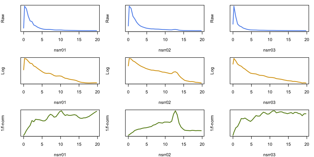
We can then use R basic plotting commands to generate spectra for the
three individuals (columns) corresponding to the raw, unnormalized
spectra showing a 1/f trend (top row), the log-scaled spectra, which
show more of a linear trend (middle row), and the normalized spectra
(bottom row). Whereas we would not expect these spectra to be
completely flat (e.g. certainly, if bandpass filters have already been
applied to the data), which the range of ~5 to 20 Hz the baselines
are relatively flat, and arguably the "peaks" (for nsrr02 around
13 Hz) are visibly clearer.
par( mfrow=c(3,3) , yaxt='n' , mar=c(4,4,1,1) )

for (i in ids) {
plot( pre$F[ pre$ID == i ] , pre$PSD[ pre$ID == i ] ,
 type="l" , lwd=2 , col="cornflowerblue" , ylab="Raw" , xlab=i )  }

for (i in ids) {
plot( pre$F[ pre$ID == i ] , 10*log10( pre$PSD[ pre$ID == i ] ),
 type="l" , lwd=2 , col="goldenrod" , ylab="Log" , xlab=i)  }

for (i in ids) {
plot( post$F[ post$ID == i ] , post$PSD[ post$ID == i ] ,
 type="l" , lwd=2 , col="olivedrab" , ylab="1/f-norm" , xlab=i)  }
TV
Applies of fast algorithm for 1D total variation denoising
The TV is a wrapper around the algorithm described
here.
In lunaC it operates on EDF channels, modifying
the in-memory representation of the signal.
Note
Given that this is not something one typically wants to
perform on raw physiological signals, a more common use-case may
be via lunaR however, where the ldenoise()
function provides a simple interface for any time series.
It is mentioned here only for completeness.
Parameters
| Parameter | Example | Description |
|---|---|---|
sig |
sig=EEG |
Optional specification of signals (otherwise applied to all signals) |
lambda |
lambda=10 |
Smoothing parameter (0 to infinity) |
See the description of ldenoise() for using
this function with lunaR. Higher values of lambda put more weight
on minimizing variation in the new signal, i.e. producing a more
flattened representation. The exact choice of lambda will depend on
the numerical scale of the data as well as its variability and the
goal of the analysis.
Outputs
No output other than modifying the in-memory representation of the signal.
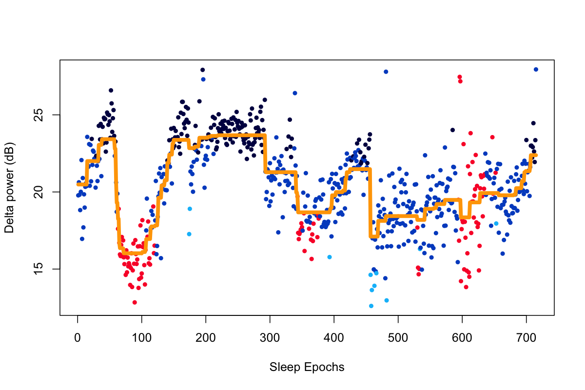
Example
Using lunaR to plot delta power across sleep epochs
and fit a de-noised line using ldenoise() (which invokes TV), to the
nsrr02 individual from the tutorial dataset:
library(luna)
sl <- lsl("s.lst")
lattach(sl,2)
k <- leval( "MASK if=wake & RE & PSD sig=EEG epoch dB" )
d <- k$PSD$B_CH_E
d <- d[ d$B == "DELTA" , ]
Also get sleep stages via the lstages() function:
ss <- lstages()
Using ldenoise(), we can fit a de-noised line, with lambda of 10 in this particular case:
d1 <- ldenoise( d$PSD , lambda = 10 )
Plotting the original and de-noised versions, also using the
convenience lstgcols() function:
plot( d$PSD, col=lstgcols(ss), pch=20, xlab="Sleep Epochs", ylab="Delta power (dB)" )
lines( d1 , lwd=5 , col="orange" )
ACF
Compute the autocorrelation function for a signal
Parameters
| Parameter | Example | Description |
|---|---|---|
sig |
sig=EEG |
Optional specification of signals (otherwise applied to all signals) |
lag |
lag=200 |
Maxmimum lag (in sample units) |
Output
ACF per channel (strata: CH x LAG)
| Variable | Description |
|---|---|
SEC |
Lag in seconds |
ACF |
Autocorrelation |
Example
To estimate the ACF for an example EEG, ECG and EMG channel, for up to 3 seconds lag
(here assuming all channels are sampled at 100 Hz, and so a lag of 300):
luna s.lst 1 -o out.db -s 'ACF sig=EEG,ECG,EMG lag=300'
ACF function, conditional on CH and LAG strata
(here putting different channels in different columns (-c CH) and different lags in different
rows (-r LAG):
destrat out.db +ACF -c CH -r LAG > o.txt
o.txt, SEC.CH_EEG on the x-axis, and ACF.CH_EEG on the y-axis), we see
strong, regular autocorrelations, with peaks at periodically recuring intervals (top row of plots below).
These would be indicative of artifact in EEG, ECG or EMG channels: indeed, in this particular case (which
is the first tutorial EDF), there is considerable artifact at the end of the recording (i.e.
with spectral peaks at 25 Hz and 12.5 Hz, reflecting harmonics of electrical noise artifacts).
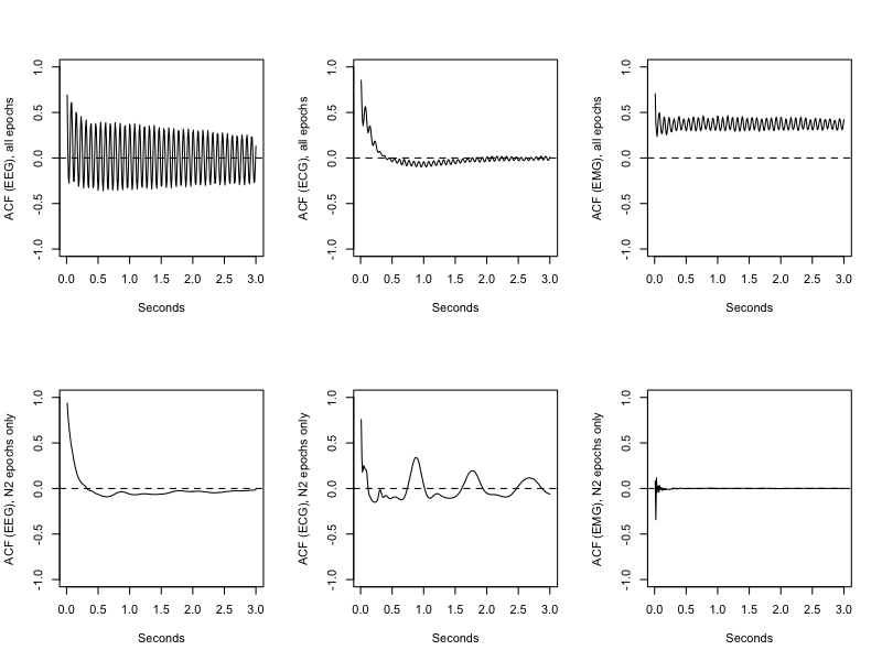
If we repeat the analysis just looking at sleep (N2) epochs (i.e. just a quick way to chop off the particularly noisy part of the recording), we see quite different ACF signatures, which are more characteristic of typical EEG, ECG and EMG respectively.
luna s.lst 1 -o out.db -s 'MASK ifnot=NREM2 & RE & ACF sig=EEG,ECG,EMG lag=300'