A deeper dive
In this third section of the tutorial, we use Luna to calculate some typical metrics of interest for sleep studies, including:
- how basic statistics vary across the night
- measures of sleep macro-architecture
- filtering and artifact detection in the EEG
- spectral analysis using fast Fourier transforms
- spindle detection using wavelets
Epoch-level summaries
Returning to the STATS command described above, here we use it
with the epoch option, in order to generate per-epoch statistics.
This section also illustrates working with the text output format.
luna s.lst 2 sig=EMG,ECG -s 'EPOCH & STATS epoch' > res.txt
===================================================================
+++ luna | v0.26.0, 11-Nov-2021 | starting 01-Dec-2021 11:08:09 +++
===================================================================
input(s): s.lst
output  : .
signals : ECG EMG
commands: c1    EPOCH
        : c2    STATS   epoch=T

___________________________________________________________________
Processing: nsrr02 [ #2 ]
 duration: 09.57.30 | 35850 secs | clocktime 21.18.06 - 07.15.36

 signals: 2 (of 14) selected in a standard EDF file
  ECG | EMG

 annotations:
  Arousal (x51) | Hypopnea (x101) | N1 (x11) | N2 (x399)
  N3 (x185) | Obstructive_Apnea (x5) | R (x120) | SpO2_artifact (x34)
  SpO2_desaturation (x66) | W (x480)

 variables:
  ecg=ECG | emg=EMG | id=nsrr02
 ..................................................................
 CMD #1: EPOCH
   options: sig=ECG,EMG
 set epochs, length 30 (step 30, offset 0), 1195 epochs
 ..................................................................
 CMD #2: STATS
   options: epoch=T sig=ECG,EMG
 processing ECG ...
 processing EMG ...

___________________________________________________________________
...processed 1 EDFs, done.
...processed 1 command set(s),  all of which passed
-------------------------------------------------------------------
+++ luna | finishing 01-Dec-2021 11:08:14                       +++
===================================================================
This command was applied only to the second EDF in the sample-list
(i.e. the 2 argument), and only to the ECG and EMG signals.
After defining 30-second epochs (the default from the EPOCH command),
it generates basic statistics per-epoch (the epoch option for the
STATS command), as well as entire-signal summaries. Note that 1195
epochs are generated, which corresponds to the stated duration of 9
hours, 57 and a half minutes (i.e. ( 9 * 60 + 57 ) * 2 + 1 = 1195).
The first few lines of res.txt are as follows:
nsrr02   EPOCH   .        .   NE       1195
nsrr02   EPOCH   .        .   DUR      30
nsrr02   EPOCH   .        .   INC      30
nsrr02   STATS   CH/ECG   1   MAX      1.25
nsrr02   STATS   CH/ECG   1   MIN     -0.651961
nsrr02   STATS   CH/ECG   1   MEAN     0.00506797
nsrr02   STATS   CH/ECG   1   SKEW     1.68822
nsrr02   STATS   CH/ECG   1   MEDIAN   0.0343137
nsrr02   STATS   CH/ECG   1   RMS      0.271051
nsrr02   STATS   CH/ECG   2   MAX      1.25
...
.)
are from the EPOCH command. The subsequent lines are
the per-epoch values from the STATS command: e.g. the mean is 0.00506797
for the first epoch.
This format is designed to be easily parsed and read by other software. For example, to use R to plot the per-epoch RMS values of the ECG, we might use the following (from within R):
d <- read.table( "res.txt" , header=F , sep="\t" , stringsAsFactors=F )
Hint
As you'll see in the next section of this tutorial, it is now possible to read lunout databases directly into R
After loading the data, it is convenient to relabel the 6 columns to have sensible names:
names(d) <- c( "ID" , "COMM" , "STRATA" , "T" , "VAR" , "VAL" )
Our goal is to generate a plot of per-epoch RMS for the ECG. We can
extract these values by filtering rows where VAR equals "RMS",
when T is not ".", and when STRATA is "CH/ECG":
d <- d[ d$STRATA == "CH/ECG" & d$T != "." & d$VAR == "RMS" , ]
We can confirm that this produces the expected number of rows/epochs:
dim(d)
[1] 1195 6
We need to ensure that the epoch and value fields are treated as numeric data points:
d$T <- as.numeric(d$T)
d$VAL <- as.numeric(d$VAL)
As a sanity-check, we can view the structure of the data frame:
str(d)
'data.frame':   1195 obs. of  6 variables:
  $ ID    : chr  "nsrr02" "nsrr02" "nsrr02" "nsrr02" ...
  $ COMM  : chr  "STATS" "STATS" "STATS" "STATS" ...
  $ STRATA: chr  "CH/ECG" "CH/ECG" "CH/ECG" "CH/ECG" ...
  $ T     : num  1 2 3 4 5 6 7 8 9 10 ...
  $ VAR   : chr  "RMS" "RMS" "RMS" "RMS" ...
  $ VAL   : num  0.271 0.279 0.268 0.264 0.265 ...
To plot these per-epochs values:
plot( d$T , d$VAL , ylab = "RMS(ECG)" , xlab = "Epoch" , pch=20 )
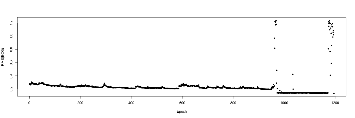
Clearly there are a number of extreme points towards the end of the
recording, presumably indicating bad data after the subject woke for
the final time that night. We can confirm this by indicating the
manually-annotated sleep stage for each point. Going back to the
command line (type q() to get out of R, or even better, run the next
couple of Luna commands in a separate window to keep the R session
open), we can use Luna to extract sleep stages (using the STAGE
command) in a format that can be read into R:
luna s.lst 2 -o ss.db -s STAGE
ss.txt:
destrat ss.db +STAGE -r E -v STAGE > ss.txt
We then load this sleep stage information into R as follows, which indicates that we have the expected number of epochs:
ss <- read.table( "ss.txt" , header=T )
dim(ss)
[1] 1195 3
This is the breakdown of epochs by each sleep stage for this individual:
table(ss$STAGE)
 N1  N2  N3   R   W
 11 399 185 120 480
If you previously closed the R session, you'll need to rerun the
commands to create the d data-frame. Then, plotting epochs colored by
sleep stage, we indeed confirm that the end aberrant epochs are all
wake: (plot not shown).
plot( d$T , d$VAL  , ylab = "RMS(ECG)" , xlab = "Epoch" , pch=20 , col = as.factor( ss$STAGE  ) )
cols <- sort(unique(ss$STAGE))
legend("topleft",legend=cols , fill = as.factor( cols ) )
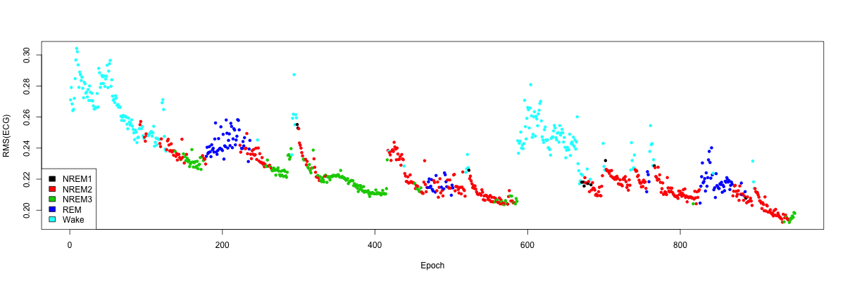
Simply ignoring these final points (which roughly corresponds to looking only up to the 950th epoch in this example), we can generate a clearer plot of how the RMS of the ECG varies across the night in this individual, which tracks with the progression of sleep and wake in a semi-predictable manner:
inc <- 1:950
plot( d$T[inc], d$VAL[inc], ylab="RMS(ECG)", xlab="Epoch", pch=20, col=as.factor(ss$STAGE[inc]) )
legend("bottomleft",legend=cols , fill = as.factor( cols ) )
Hypnograms
Given a set of epoch-based staging values, the HYPNO command
produces a series of statistics that describe different aspects of
sleep macro-architecture.
luna s.lst -o stage.db -s 'EPOCH & HYPNO epoch'
This generate a large number of variables, as described here.
There are various different strata groups in the output from STAGE:
destrat stage.db
--------------------------------------------------------------------------------
stage.db: 2 command(s), 3 individual(s), 66 variable(s), 107919 values
--------------------------------------------------------------------------------
  command #1:   c1  Thu Aug 13 13:40:56 2020    EPOCH   sig=*
  command #2:   c2  Thu Aug 13 13:40:56 2020    HYPNO   sig=*
-------------------------------------------------------------------------
distinct strata group(s):
 commands  : factors   : levels      : variables
-----------:-----------:-------------:---------------------------
 [EPOCH]   : .         : 1 level(s)  : DUR GENERIC INC NE OFFSET
           :           :             :
 [HYPNO]   : .         : 1 level(s)  : CONF E0_START E1_LIGHTS_OFF E2_SLEEP_ONSET
           :           :             : E3_SLEEP_MIDPOINT E4_FINAL_WAKE
           :           :             : E5_LIGHTS_ON E6_STOP EINS FIXED_LIGHTS
           :           :             : FIXED_SLEEP FIXED_WAKE FWT HMS0_START
           :           :             : HMS1_LIGHTS_OFF HMS2_SLEEP_ONSET
           :           :             : HMS3_SLEEP_MIDPOINT HMS4_FINAL_WAKE
           :           :             : HMS5_LIGHTS_ON HMS6_STOP LOST LOT
           :           :             : LZW LZW3 NREMC NREMC_MINS OTHR
           :           :             : POST PRE REM_LAT REM_LAT2 SE SFI
           :           :             : SINS SME SOL SOL_PER SPT SPT_PER
           :           :             : T0_START T1_LIGHTS_OFF T2_SLEEP_ONSET
           :           :             : T3_SLEEP_MIDPOINT T4_FINAL_WAKE
           :           :             : T5_LIGHTS_ON T6_STOP TGT TIB TI_RNR
           :           :             : TI_S TI_S3 TRT TST TST_PER TWT
           :           :             : WASO
           :           :             :
 [HYPNO]   : E         : (...)       : AFTER_GAP CLOCK_HOURS CLOCK_TIME
           :           :             : CYCLE CYCLE_POS_ABS CYCLE_POS_REL
           :           :             : E_N1 E_N2 E_N3 E_REM E_SLEEP E_WAKE
           :           :             : E_WASO FLANKING FLANKING_ALL MINS
           :           :             : N2_WGT NEAREST_WAKE OSTAGE PCT_E_N1
           :           :             : PCT_E_N2 PCT_E_N3 PCT_E_REM PCT_E_SLEEP
           :           :             : PERIOD PERSISTENT_SLEEP POST PRE
           :           :             : SPT STAGE STAGE_N START_SEC TOT_NR2R
           :           :             : TOT_NR2W TOT_R2NR TOT_R2W TOT_W2NR
           :           :             : TOT_W2R TR_NR2R TR_NR2W TR_R2NR
           :           :             : TR_R2W TR_W2NR TR_W2R WASO
           :           :             :
 [HYPNO]   : C         : 6 level(s)  : NREMC_MINS NREMC_N NREMC_NREM_MINS
           :           :             : NREMC_OTHER_MINS NREMC_REM_MINS
           :           :             : NREMC_START
           :           :             :
 [HYPNO]   : SS        : 11 level(s) : BOUT_05 BOUT_10 BOUT_MD BOUT_MN
           :           :             : BOUT_MX BOUT_N DENS MINS PCT TA
           :           :             : TS
           :           :             :
 [HYPNO]   : N         : 141 level(s): FIRST_EPOCH LAST_EPOCH MINS STAGE
           :           :             : START STOP
           :           :             :
 [HYPNO]   : PRE POST  : 9 level(s)  : N P P_POST_COND_PRE P_PRE_COND_POST
           :           :             :
           :           :             :
-----------:-----------:-------------:---------------------------
The first (.) HYPNO group is a set of variables with no
stratifiers: that is, simply one value per individual/EDF, such as
Total Sleep Time (TST).
Stage durations are stratifed by SS (sleep stage).
To view the number of minutes of each sleep stage for the three individuals,
NREMC, we can use:
destrat stage.db +HYPNO -c SS/N1,N2,N3,R -v MINS
ID       MINS.SS_N1   MINS.SS_N2    MINS.SS_N3    MINS.SS_R
nsrr01   54.5         261.5         8.5           119
nsrr02   5.5          199.5         92.5          60
nsrr03   26           187.5         10.5          0
To view cycle-level variables (C factor), we can use the following
to see the duration (in minutes) and start (in epoch number):
destrat stage.db +HYPNO -r C -v NREMC_START NREMC_MINS
ID       C    NREMC_MINS  NREMC_START
nsrr01   1    45          87
nsrr01   2    100.5       184
nsrr01   3    47          451
nsrr01   4    77.5        654
nsrr01   5    60          819
nsrr01   6    50          956
nsrr02   1    72.5        92
nsrr02   2    133         237
nsrr02   3    42          503
nsrr02   4    105.5       675
nsrr02   5    32.5        887
nsrr03   1    69          118
nsrr03   2    74          312
nsrr03   3    137.5       630
To illustrate extracting epoch-level information: here we consider the
designated sleep stage (STAGE variable), along with the time
(CLOCK_TIME) and a measure of how many nearby epochs had the same
stage (FLANKING). By default, FLANKING treats all three NREM stages
as similar for this particular analysis, unless the option flanking-collapse-nrem=F
is passed to HYPNO. The latter is the minimum number of
contiguous epochs, either forwards or backwards in time, that are
similar to the index epoch (truncated at the start and end of the
recording). In other words, selecting epochs with 3 or more for this
variable means that there are at least 3 epochs before and 3 epochs
after with a similar stage. This can be used to select periods of
sleep that are less likely to contain stage transitions, for example.
destrat stage.db +HYPNO -i nsrr01 -r E -v STAGE FLANKING CLOCK_TIME
ID       E      CLOCK_TIME   FLANKING  STAGE
nsrr01   1      21:58:17     0         W
nsrr01   2      21:58:47     1         W
nsrr01   3      21:59:17     2         W
nsrr01   4      21:59:47     3         W
nsrr01   5      22:00:17     4         W
nsrr01   6      22:00:47     5         W
nsrr01   7      22:01:17     6         W
nsrr01   8      22:01:47     7         W
nsrr01   9      22:02:17     8         W
nsrr01   10     22:02:47     9         W
nsrr01   11     22:03:17     10        W
 ... cont'd ...
nsrr01  183     23:29:17     0         N1
nsrr01  184     23:29:47     0         N2
nsrr01  185     23:30:17     0         W
nsrr01  186     23:30:47     0         N1
nsrr01  187     23:31:17     1         N2
nsrr01  188     23:31:47     2         N2
nsrr01  189     23:32:17     3         N2
nsrr01  190     23:32:47     4         N2
nsrr01  191     23:33:17     5         N2
nsrr01  192     23:33:47     6         N2
nsrr01  193     23:34:17     7         N2
nsrr01  194     23:34:47     8         N2
nsrr01  195     23:35:17     9         N2
nsrr01  196     23:35:47     10        N2
nsrr01  197     23:36:17     11        N2
nsrr01  198     23:36:47     10        N2
nsrr01  199     23:37:17     9         N2
nsrr01  200     23:37:47     8         N2
nsrr01  201     23:38:17     7         N2
nsrr01  202     23:38:47     6         N2
nsrr01  203     23:39:17     5         N2
nsrr01  204     23:39:47     4         N2
nsrr01  205     23:40:17     3         N2
nsrr01  206     23:40:47     2         N2
nsrr01  207     23:41:17     1         N2
nsrr01  208     23:41:47     0         N2
nsrr01  209     23:42:17     0         W
nsrr01  210     23:42:47     0         N2
 ... cont'd
Epoch-level masks
To illustrate applying different epoch-level masks, consider the following (somewhat unrealistic) example - to select epochs that:
- occur between 11pm and 3am
- are in persistent sleep as defined above (i.e. at least 10 minutes of sleep prior)
- are during stage 2 NREM sleep
- do not contain any apnea or hypopnea events
The following Luna command script (cmd/third.txt) shows one way of doing this, leveraging the
ability of HYPNO to add annotations on-the-fly (to define persistent sleep):
% with `annot`, HYPNO will add annotations to the EDF starting h_
% and will include the epoch-level annotation h_persistent_sleep
HYPNO annot

% not needed, but start by ensuring mask is reset
MASK none

% first select epochs based on clock-time
MASK hms=23:00:00-03:00:00

% equivalently - at resolution of 1hr at least - could have
% used annotations added by `HYPNO annot`
%MASK mask-ifnot=h_clock_23,h_clock_00,h_clock_01,h_clock_02

% next, include only if in persistent sleep
MASK mask-ifnot=h_persistent_sleep

% select only N2 epochs
MASK mask-ifnot=N2

% and reject epochs with any respiratory event
MASK mask-if=Obstructive_Apnea,Hypopnea

% finally, output the mask
DUMP-MASK
The above first runs HYPNO (which also epochs the data in 30-second
epochs) but adds the flag annot which tells HYPNO to add a series
of annotations to the recording, largely based upon the hynogram.
By default, these start with the prefix h_ and include one that
defines (at an epoch-level) persistent sleep, called
h_persistent_sleep.
Next, although not strictly necessary, we clear the mask (i.e. to include all epochs). We
then use the hms flag to mask any epoch outside of the specified
range. (Actually, this includes any epoch that has any overlap with
the interval between 23:00:00 and 03:00:00, i.e. so it will also
include a 30-second epoch that starts at 22:59:47, for example. If you
require more precise timing, should should set epoch duration to be 1
second, not 30 seconds, for example, when running the MASK hms
command.)
Info
You must use 24 hour hh:mm:ss notation, so 11pm is 23:00:00.
As shown above, HYPNO annot also emits some annotations corresponding to clock-times,
and we could have used that MASK statement instead to achieve the same effect.
It next masks any epochs that are not labelled as h_persistent_sleep.
Next, it masks any epoch that is not stage 2 NREM sleep (annotation
N2).
Note
Here we used the mask-ifnot rather than ifnot flag: the
difference is that the former will not unmask N2 epochs that
were previously masked. Remember:
- To mask or set the mask to true means to exclude that epoch.
- To unmask or set the mask to false mean to include that epoch.
See the page on masks for a detailed description of how
the MASK syntax works in Luna.
Finally, it masks any epochs that contain at least one apnea or
hypopnea event, using the labels Obstructive_Apnea and Hypopnea as
they appear in the Luna console output (i.e. with an underscore
replacing the space).
Let's run this command, just for nsrr01, in order to study the output sent to the console
that describes the masking process (i.e. we'll ignore the output in out.db):
luna s.lst id=nsrr01 -o out.db < cmd/third.txt
MASK stage. First, the hypnogram derived
annotations are added from running HYPNO, with a note that
these will have a prefix h_:
 CMD #1: HYPNO
   options: annot sig=*
  set epochs to default 30 seconds, 1364 epochs
  set 0 leading/trailing sleep epochs to '?' (given end-wake=120 and end-sleep=5)
  creating hypnogram-derived annotations, with prefix h
ANNOTS command or see the documentation
page for HYPNO. Next, all epochs are included (with
the none mask option):
 CMD #2: MASK
  set masking mode to 'mask' (default)
  reset all 1364 epochs to be included
Next, epochs between 11pm and 3am are included, all other epochs are masked. As a sanity check, from epoch 124 to 604 inclusive is 481 epochs, which is 4 hours and 30 seconds (i.e. this includes an extra epoch that started at 22:59:47 and so still overlaps the 11pm-3am interval):
 CMD #3: MASK
  selecting epochs from 124 to 604; selecting from set of 481 epochs; 883 newly masked, 0 unmasked, 0 unchanged
  total of 481 of 1364 retained
At this point there are 481 unmasked epochs, although because we
have not yet issued any RESTRUCTURE
command, the effective duration of the in-memory EDF is still 1364
epochs. We next further mask epochs that are not in persistent sleep:
 CMD #4: MASK
  annots: h_persistent_sleep
  applied annotation mask for 1 annotation(s)
  644 epochs match; 209 newly masked, 0 unmasked, 1155 unchanged
  total of 272 of 1364 retained
Based on this, it implies that 209 epochs are within the 11pm to 3am window but not
in persistent sleep, as they are newly masked. Only those epochs have their
status changed (i.e. because we've set this MASK commands up to
only ever mask, not to unmask, epochs), leaving us with 272
epochs:
Next, we further mask based on not being in N2 sleep, which drops us to 235 epochs:
 CMD #5: MASK
  annots: N2
  applied annotation mask for 1 annotation(s)
  523 epochs match; 37 newly masked, 0 unmasked, 1327 unchanged
  total of 235 of 1364 retained
Finally, we screen for matching any apnea or hypopnea event, which takes us down to 86 epochs:
 CMD #6: MASK
  annots: Hypopnea Obstructive_Apnea
  applied annotation mask for 2 annotation(s) (using or-matching across multiple annotations)
  558 epochs match; 149 newly masked, 0 unmasked, 1215 unchanged
  total of 86 of 1364 retained
The final command writes the mask status (masked or not) to the
output. In practice, we would now likely perform a RE command to
restructure the dataset, and then run subsequent commands or output a
new EDF, etc.
Manipulating EDFs
Here we give an overview of filtering, resampling, relabelling, re-referencing and re-writing signal data.
The following command script (cmd/fourth.txt) illustrates the above features:
mV
RESAMPLE sr=100
FILTER bandpass=0.3,35 ripple=0.02 tw=1
REFERENCE ref=EEG1 sig=EEG2
WRITE edf-tag=v2 edf-dir=newedfs/ sample-list=new.lst
Using the following Luna command (note use of the parameter file
cmd/vars.txt to define new labels EEG1 and EEG2):
luna s.lst @cmd/vars.txt sig=EEG1,EEG2 < cmd/fourth.txt
Processing: nsrr01 [ #1 ]
 duration: 11.22.00 | 40920 secs | clocktime 21.58.17 - 09.20.17

 signals: 2 (of 14) selected in a standard EDF file:
  EEG2 | EEG1

 annotations:
  Arousal (x194) | Hypopnea (x361) | N1 (x109) | N2 (x523)
  N3 (x17) | Obstructive_Apnea (x37) | R (x238) | SpO2_artifact (x59)
  SpO2_desaturation (x254) | W (x477)

 variables:
  eeg=EEG2,EEG1 | id=nsrr01
 ..................................................................
 CMD #1: mV
   options: sig=EEG1,EEG2
  rescaled EEG1 to mV
  rescaled EEG2 to mV
 ..................................................................
 CMD #2: RESAMPLE
   options: sig=EEG1,EEG2 sr=100
  resampling channel EEG1 from sample rate 125 to 100
  resampling channel EEG2 from sample rate 125 to 100
 ..................................................................
 CMD #3: FILTER
   options: bandpass=0.3,35 ripple=0.02 sig=EEG1,EEG2 tw=1
  filtering channel(s): EEG1 EEG2
 ..................................................................
 CMD #4: REFERENCE
   options: ref=EEG1 sig=EEG2
  referencing EEG2 with respect to EEG1
 ..................................................................
 CMD #5: WRITE
   options: edf-dir=newedfs/ edf-tag=v2 sample-list=new.lst sig=EEG1,EEG2
  appending newedfs/learn-nsrr01-v2.edf to sample-list new.lst (dropping any annotations)
  no epoch mask set, no restructuring needed
nsrr01  WRITE   .   .   NR1 40920
nsrr01  WRITE   .   .   NR2 40920
nsrr01  WRITE   .   .   DUR1    40920
nsrr01  WRITE   .   .   DUR2    40920
  data are not truly discontinuous
  writing as a standard EDF
  writing 2 channels
  saved new EDF, newedfs/learn-nsrr01-v2.edf

___________________________________________________________________
This selects only the two EEG signals, based on their aliases EEG1 and
EEG2. the mV command rescales any signals in uV and V units to
mV, changing the EDF headers appropriately too. The RESEAMPLE
command takes an argument sr which is the new sampling rate
(i.e. set to 100Hz here). The FILTER command designs and applies a
FIR filter with transition frequencies at 0.3 and 35 Hz.
The REFERENCE command re-references the signal data -- in this
example, for illustration of the syntax only, we reference EEG2
relative to EEG1 (i.e. subtract EEG1 values from EEG2). Signals must
have the same sampling rate to be referenced. Multiple,
comma-delimited signals can be given as the ref, in which case the
average of those values is used as the reference; if multiple signals
are given for the sig command, then each signal is re-referenced
with respect to whatever ref was specified.
Finally, the WRITE command generates a new EDF, that will reflect
these changes. The edf-tag value is appended to the original
filename for the EDF, and it is written to a directory edf-dir (if
this doesn't exist, it will be created). A new sample-list new.lst
is also generated, with each newly generated EDF being appended to it.
(Note, values are only appended to the sample-list, to facilitate
running Luna in parallel, so if new.lst already existed and was not
empty, you might want to delete that file before running the above.)
We can confirm that the new sample list is as expected:
cat new.lst
nsrr01     newedfs/learn-nsrr01-v2.edf
nsrr02     newedfs/learn-nsrr02-v2.edf
nsrr03     newedfs/learn-nsrr03-v2.edf
We can also inspect the new sets of EDFs, using the SUMMARY command on new.lst:
luna new.lst id=nsrr01 -s SUMMARY
EDF filename   : newedfs/learn-nsrr01-v2.edf
Patient ID     :
Recording info :
Start date     : 01.01.85
Start time     : 21:58:17

# signals      : 2
# records      : 40920
Duration       : 1

Signal 1 : [EEG2]
       # samples per record : 100
       transducer type      :
       physical dimension   : mV
       min/max (phys)       : -0.3726/0.391668
       EDF min/max (phys)   : -0.3726/0.391668
       min/max (digital)    : -32768/32767
       EDF min/max (digital): -32768/32767
       pre-filtering        :

Signal 2 : [EEG1]
       # samples per record : 100
       transducer type      :
       physical dimension   : mV
       min/max (phys)       : -0.24235/0.237407
       EDF min/max (phys)   : -0.24235/0.237407
       min/max (digital)    : -32768/32767
       EDF min/max (digital): -32768/32767
       pre-filtering        :
That is, in relation to the original SUMMARY for this individual,
the sampling rate is different, the labels have been reset to their
alias values, there are now only two signals, not 14, the units of mV
and not uV, and the min/max range is different (reflecting both the
change in scale, and the filtering and referencing).
Artifact detection
Here we detect likely artifact in EEG (and other) signals, using two approaches. The first, specific to sleep EEG, is as described by Buckelmueller et al (2006). The second is based on per-epoch statistical filtering of RMS and Hjorth parameters.
Running just for the first individual, the command file
cmd/fifth.txt contains the following:
EPOCH
MASK if=W
RESTRUCTURE
FILTER bandpass=0.3,35 ripple=0.02 tw=1
SIGSTATS epoch
After filtering the signal to consider only sleep epochs, and
filtering the signal to remove very slow and fast rhythms, we use the
SIGSTATS command to generate Hjorth parameters (and also RMS) for a
signal, both overall (i.e. all sleep epochs) and per-epoch (by virtue
of the epoch option). We run Luna and save the results in
artifact.db, only for a single EEG channel for now:
luna s.lst 1 sig=EEG -o artifact.db < cmd/fifth.txt
Viewing the contents of artifact.db:
destrat artifact.db
--------------------------------------------------------------------------------
artifact.db: 5 command(s), 1 individual(s), 16 variable(s), 2677 values
--------------------------------------------------------------------------------
  command #1:   c1  Thu Aug 13 13:45:19 2020    EPOCH   sig=EEG
  command #2:   c2  Thu Aug 13 13:45:19 2020    MASK    if=W sig=EEG
  command #3:   c3  Thu Aug 13 13:45:19 2020    RESTRUCTURE sig=EEG
  command #4:   c4  Thu Aug 13 13:45:19 2020    FILTER  bandpass=0.3,35 ripple=0.02 sig=EEG tw=1
  command #5:   c5  Thu Aug 13 13:45:20 2020    SIGSTATS    epoch=T sig=EEG
--------------------------------------------------------------------------------
distinct strata group(s):
  commands      : factors           : levels        : variables
----------------:-------------------:---------------:---------------------------
  [EPOCH]       : .                 : 1 level(s)    : DUR GENERIC INC NE OFFSET
                :                   :               :
  [MASK]        : EMASK             : 1 level(s)    : MASK_MODE MATCH_LOGIC MATCH_TYPE
                :                   :               : N_MASK_SET N_MASK_UNSET N_MATCHES
                :                   :               : N_RETAINED N_TOTAL N_UNCHANGED
                :                   :               :
                :                   :               :
  [RESTRUCTURE] : .                 : 1 level(s)    : DUR1 DUR2 NA NR1 NR2 NS
                :                   :               :
  [SIGSTATS]    : CH                : 1 level(s)    : H1 H2 H3
                :                   :               :
  [SIGSTATS]    : E CH              : (...)         : H1 H2 H3
                :                   :               :
----------------:-------------------:---------------:---------------------------
The SIGSTATS command produces Hjorth parameters (H1, H2 and H3) both
overall (CH strata group) and per-epoch (E CH strata group). To
see the overall values:
destrat artifact.db +SIGSTATS -r CH -p 2
ID      CH   H1     H2    H3
nsrr01  EEG  78.38  0.35  0.83
To save all per-epoch values to a file res.txt:
destrat artifact.db +SIGSTATS -r CH E > res.txt
One can load this file in R, for example, to view the per-epoch distribution (we do this below also).
As well as viewing these statistics, we can use them to flag likely
artifacts, by considering values that are statistical outliers in the
per-epoch distribution. If we consider a new command script, below
(and cmd/sixth.txt in the tutorial folder), we add the mask option
to the SIGSTATS command, and specify a set of thresholds: 3,3,3
means to iteratively remove epochs that are more than 3 standard
deviations above or below the mean. We also add the ARTIFACTS
command beforehand, which implements the Buckelmueller et
al. filtering referenced above. Note that the SIGSTATS command will
only operate on unmasked values (the prior ARTIFACTS command will
have masked some).
EPOCH
MASK if=W
RESTRUCTURE
FILTER bandpass=0.3,35 ripple=0.02 tw=1
ARTIFACTS mask
CHEP-MASK ep-th=3,3,3 epoch
CHEP epochs
DUMP-MASK
Running this new script, which ends by saving the current mask, we see the following:
luna s.lst 1 sig=EEG -o mask.db < cmd/sixth.txt
 ... cont'd ...
 CMD #5: ARTIFACTS
   options: mask=T sig=EEG
  masked 12 of 887 epochs, altering 12
 ..................................................................
 CMD #6: CHEP-MASK
   options: ep-th=3,3,3 epoch=T sig=EEG
  within-channel/between-epoch outlier detection, ep-th = 3,3,3
   iteration 1: removed 21 channel/epoch pairs this iteration (21 in total)
   iteration 2: removed 9 channel/epoch pairs this iteration (30 in total)
   iteration 3: removed 5 channel/epoch pairs this iteration (35 in total)
 ..................................................................
 CMD #7: CHEP
   options: epochs=T sig=EEG
  masking epochs with >0% masked channels: 35 epochs
  CHEP summary:
   35 of 887 channel/epoch pairs masked (4%)
   35 of 887 epochs with 1+ masked channel, 35 with all channels masked
   1 of 1 channels with 1+ masked epoch, 0 with all epochs masked
 ..................................................................
 ... cont'd ...
That is, the first approach to artifact detection removes 12 epochs;
the second approach (which itself comprises three iterations) removes
a total of 35 additional epochs. We can extract the mask (output by
the DUMP-MASK command)
destrat mask.db +DUMP-MASK -r E -v EMASK > mask.txt
This has 888 rows: one header plus the 887 non-wake epochs (i.e. after
a RESTRUCTURE command, this is the "total" number of epochs left).
Loading this file, plus the previous output from SIGSTATS into R, we
can plot the per-epoch distribution of the Hjorth parameters, colored
by whether that epoch was excluded by artifact detection (run the
following in R):
 d <- read.table("res.txt",header=T,stringsAsFactors=F)
 m <- read.table("mask.txt",header=T,stringsAsFactors=F)
 m <- merge( d , m , by=c("ID","E") )

 par(mfcol=c(3,1),mar=c(4,4,1,1))
 plot( m$E , m$H1 , pch = 20 , xlab="Epoch" , ylab="H1" , col = m$EMASK + 1)
 plot( m$E , m$H2 , pch = 20 , xlab="Epoch" , ylab="H2" , col = m$EMASK + 1)
 plot( m$E , m$H3 , pch = 20 , xlab="Epoch" , ylab="H3" , col = m$EMASK + 1)
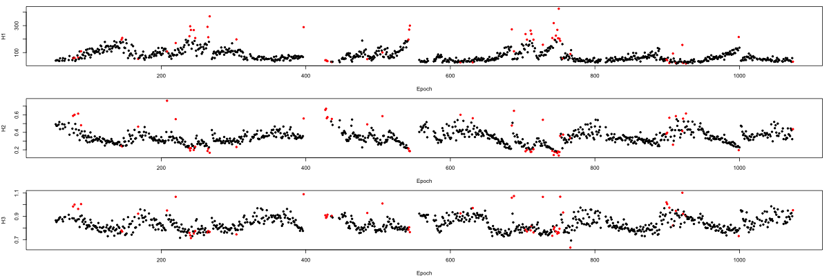
In practice, given the heterogeneous nature of sleep signals, naturally it may be preferable to perform stage-specific artifact detection, or only remove very aberrant signals based on global outlier status.
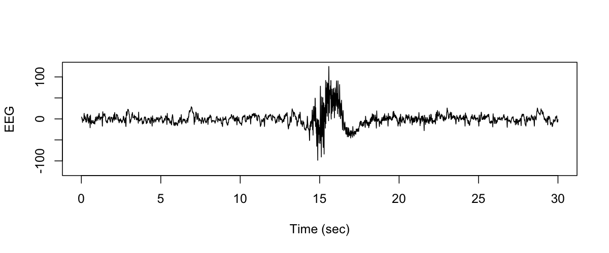
To examine one of the removed epochs more closely (we can use scope
as below, also), here we illustrate using commands such as DUMP and
MATRIX to obtain simple, plain-text signal data. This extracts the
EEG signal only, for the first individual's epoch 220. (This was one
of the flagged epochs, as you can see by examining the output of
DUMP-MASK above.
luna s.lst 1 sig=EEG -s 'EPOCH & MASK epoch=220 & MATRIX file=eeg.txt minimal'
This is a plain-text file with one number (sample-point) per row. We expect 30 times 125 = 3750 rows, for a single 30-sec epoch of signal sampled at 125 Hz. In R:
s <- scan("eeg.txt")
Read 3750 items
We can then generate a plot of this signal, e.g. :
plot( seq(1/125,30,1/125), s, type="l", ylim=c(-125, 125 ) ,
      xlab="Time (sec)" , ylab="EEG" )
Info
lunaR provides a far easier means to directly import raw signal data into R, that does not involve intermediate text file; we'll consider this explicitly in the next tutorial section.
Spectral and spindle analyses
To generate the EEG power density spectrum for each individual, say
during stage 2 NREM sleep, we can use the PSD command.
Specifically, if we had a command file as follows:
EPOCH
MASK ifnot=N2
RESTRUCTURE
FILTER bandpass=0.3,35 ripple=0.02 tw=1
ARTIFACTS mask
CHEP-MASK ep-th=3,3,3
CHEP epoch
RESTRUCTURE
PSD spectrum
then the following command should epoch the signals, only include N2 epochs, filter the EEG and attempt to remove epochs that contain gross artifact, and then calculate the power spectra, both for classical bands (delta, alpha, sigma, etc) and also for each frequency bin (subject to the resolution determined by the sampling frequency and the size of the intervals analyzed. Internally, Luna uses of Welch algorithm and FFT to estimate the PSD.
luna s.lst sig=EEG -o out.db < cmd/seventh.txt
Note
This script cmd/seventh.txt also contains two extra commands at the end
to detect spindles, which we'll describe below.
The power spectra are values implicitly stratified both by channel
(CH) and frequency (F), so we use the following command to extract
the absolute power values:
destrat out.db +PSD -r F CH -v PSD > res.psd
In R, we can read the res.psd file as follows,
d <- read.table("res.psd",header=T,stringsAsFactors=F)
head(d)
      ID  CH    F      PSD
1 nsrr01 EEG 0.50 26.09547
2 nsrr01 EEG 0.75 36.36182
3 nsrr01 EEG 1.00 39.85385
4 nsrr01 EEG 1.25 30.42863
5 nsrr01 EEG 1.50 22.48063
6 nsrr01 EEG 1.75 19.02125
We can create 3 plots, on a log-scale, of
par(mfcol=c(1,3))
ids <- unique(d$ID)
for (i in ids) plot( d$F[ d$ID == i ] , log( d$PSD[ d$ID == i ] ) ,
  type="l" , xlab="Hz" , ylab="log(uV^2/Hz)" , lwd=2,main=i)
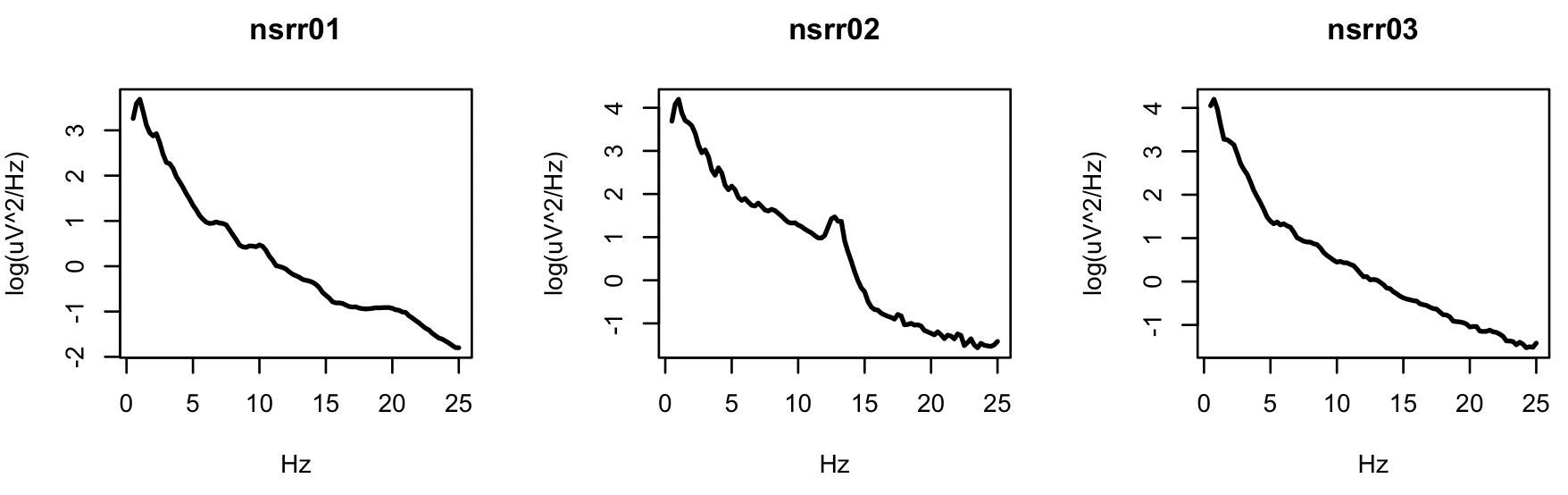
Especially for the second individual, we see the characteristic peak in the sigma band (11-15Hz), typically representing spindle activity during stage 2 NREM sleep.
As a side-note: naturally, without filtering and artifact detection, especially if including many waking epochs at the start and end of recordings, the power spectra can be very noisy, indicating many sources of (typically non-biological) artifact. For example, this command estimates the PSD without any prior filtering:
luna s.lst @cmd/vars.txt sig=EEG1,EEG2 -o psd-all.db \
   -s 'EPOCH & MASK if=W & PSD spectrum max=62'
destrat psd-all.db +PSD -r CH F -v PSD > res.psd-all
In R:
d <- read.table( "res.psd-all",header=T,stringsAsFactors=F)
par(mfrow=c(2,3))
ids <- unique(d$ID)
for (ch in c("EEG1","EEG2") )
 for (i in ids)
   plot( d$F[ d$ID == i & d$CH == ch ] , log( d$PSD[ d$ID == i & d$CH == ch ] ) ,
            type="l" , xlab="Hz" , ylab="log(uV^2/Hz)" , lwd=2,main=paste(i,ch))
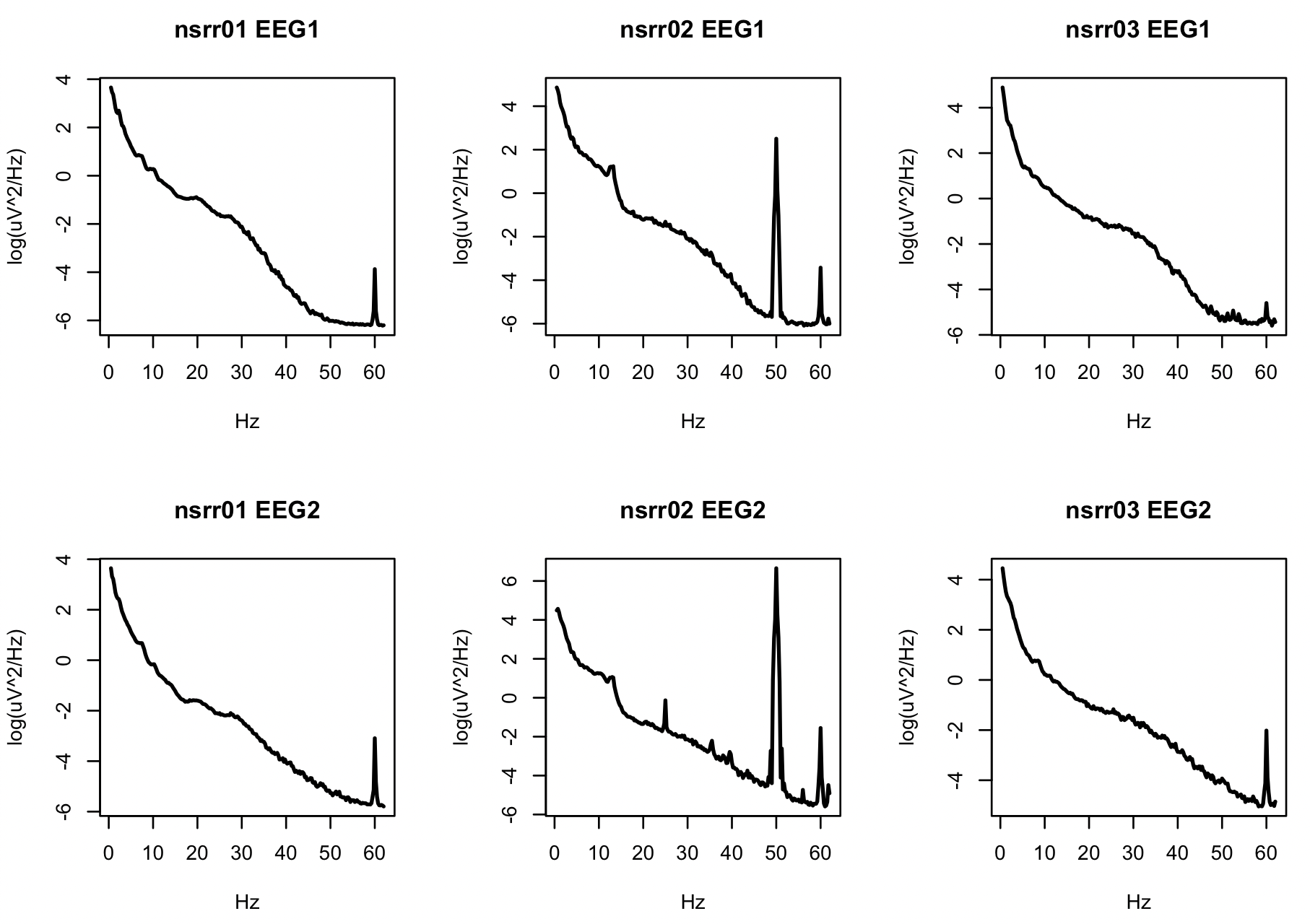
Especially for nsrr02, there is clearly a great deal of 50 and 60Hz
line noise in the signals. Visual inspection of the signals,
especially EEG2 reveals other artifacts (below). Depending on the
type of analyses one wishes to perform, careful filtering and/or
artifact detection/correction will be important.
Finally, as we noted above, the last two lines of cmd/seventh.txt
additionally instructed Luna to detect spindles and then write them to a file (where the ^ indicates the
individual ID is to be swapped in):
SPINDLES fc=11,15 annot=spindles
WRITE-ANNOTS file=spindles-^.txt annot=spindles no-specials
The fc options specify the targeted frequencies: slower spindles
at 11 Hz and faster spindles at 15 Hz. The annot options request
that an annotations be generated (for each individual) to
represent the spindle calls -- these can be used as filters.
To extract the spindle density (count per minute, DENS) we use the following command:
destrat out.db +SPINDLES -r CH -c F -v DENS -p 2
ID     CH   DENS.F_11  DENS.F_15
nsrr01 EEG  0.73       0.64
nsrr02 EEG  1.29       2.06
nsrr03 EEG  0.72       0.19
Because we added the annot option, Luna generated some annotations
that represent the spindle calls and some associated per-spindle meta-data (e.g. amplitude amp).
These are then saved in the final
command, WRITE-ANNOTS to .annot files.
head spindles-nsrr01.txt
class    instance  channel    start       stop   meta
spindles   15      EEG     2706.560   2707.176   amp=11.0679|dur=0.616|frq=13.7987|isa=0.790763|rp_mid=0.736842
spindles   11      EEG     2834.640   2835.224   amp=19.1707|dur=0.584|frq=10.274|isa=0.839118|rp_mid=0.638889
spindles   15      EEG     2868.120   2868.752   amp=12.5175|dur=0.632|frq=13.4494|isa=0.889038|rp_mid=0.410256
spindles   11      EEG     2868.832   2869.656   amp=15.9973|dur=0.824|frq=10.3155|isa=0.993035|rp_mid=0.294118
spindles   15      EEG     2870.896   2871.408   amp=13.3631|dur=0.512|frq=13.6719|isa=0.900901|rp_mid=0.730159
spindles   15      EEG     2905.008   2905.696   amp=16.0575|dur=0.688|frq=13.0814|isa=1.64327|rp_mid=0.341176
spindles   15      EEG     2949.696   2950.520   amp=19.6564|dur=0.824|frq=14.5631|isa=2.4089|rp_mid=0.578431
spindles   11      EEG     2969.200   2969.768   amp=15.1515|dur=0.568|frq=9.6831|isa=0.823499|rp_mid=0.271429
spindles   11      EEG     2978.264   2979.192   amp=14.4497|dur=0.928|frq=10.2371|isa=0.924797|rp_mid=0.365217
...
There are a large number of other options and output variables for the
SPINDLES and other commands,
described in the Reference pages of this web site.