Interval-based analyses

Command	Description
`OVERLAP`	Annotation overlap/enrichment (single-sample)
`--overlap`	Annotation overlap/enrichment (multi-sample)
`MEANS`	Signal means by annotation
`PEAKS`	Detect and cache signal peaks
`Z-PEAKS`	Detect and cache signal peaks, alternative method
`TLOCK`	Time-locked (e.g. peak-locked) signal averaging

OVERLAP

Randomisation framework to evaluate overlap/proximity between two or more sets of (multi-channel) annotations

This command calculates a series of simple overlap/proximity metrics for interval-based annotations, either in a single individual or (if using the --overlap command) multiple individuals. One or more annotation classes must be set as seeds; during randomisation, seeds are shuffled to generate empirical null distributions for evaluated metrics. Shuffling all events together largely preserves the inter-event time distribution (one exception is that annotations will "wrap" around if shuffled past the end of the analysed region (i.e. they will appear near the start of the analysis region).

Background intervals and shuffling

By default, the analysis region spans from 0 seconds (EDF start) to the end of the last annotation. Alternatively, a set of background annotations can be specified explicitly (the bg and xbg options) such that only annotations that fall within a background interval (e.g. all QC+ NREM epochs) are included. Shuffling then occurs only within each contiguous background region. Note that both test and background annotations are flattened prior to analysis, i.e. merging overlapping and contiguous annotations of the same class into a single interval/segment.

By default, seeds are shuffled by a random offset between 0 and the length of the bounding background segment. Alternatively, one can further constrain shuffling (via max-shuffle), by requiring the offsets to be no larger than X seconds (e.g. 30). This might be useful when analysing long, continuous intervals (e.g. hours): here, the rate of different events may vary over time which could result in spurious "coupling" being detected, even in the absence of any true above-chance local overlap. One caveat is that any events wrapped around (i.e. shuffled past the end of the background) may necessarily end up further away (in time) than max-shuffle.

This is a toy example of a valid shuffle for one seed class containing three events for a given channel/background region:

          background:  |-------------------|            
                       |                   |
            original:  | 111  222      33  | 
                       |                   |
            shuffled:  |---------->111  222|      33    
                       |                   |               
 annotation #3 wraps:  |      33   111  222|                   
                       |                   |
                       |-------------------|

In contrast, this shuffle would not be allowed:

          background:  |-------------------|            
                       |                   |
            original:  | 111  222      33  | 
                       |                   |
            shuffled:  |----------->111  22|2      33
                       |                   |
 illegal, splits #2:   |2  33       111  22|
                       |                   |
                       |-------------------|

Channel-specific annotations

By default, within the same channel seeds of the same class are shuffled together, whereas seeds assigned to different channels are shuffled independently. Shuffling can be modified such that all some or all seed classes/channels are shuffled together (via the align option). When shuffling, the same constraint that no event can span a background boundary will still hold. Alternatively, one can collapse all events of the same annotation class across channels, either for all (pool-channels) or some (pool-channels=A,B) annotations, i.e. effectively ignoring channel.

If a channel is specified, new annotation classes will be created for this analysis, e.g. for seed class A and channels C3 and C4, this will lead to A_C3 and A_C4.

If you wish to only test for overlap for events occurring within the same channel, add the within-channel option.

Annotations and channels

Not all annotations need be associated with a channel, either in general or with the OVERLAP command in particular. An annotation is associated with a channel is it is a channel label appears in the third column of a full-format .annot file. If this is a period (.), then no channel is associated.

Unsuitable inputs

OVERLAP keeps randomising until it finds a valid shuffle. However, if more than a certain number of unsuccessful attempts are made, Luna will give a warning. This typically means that the data are not suitable for this method. For example, if a single seed event completely spans the background interval, it will not be possible to shuffle it.

Seed metrics

OVERLAP assesses the pile-up among seeds, by enumerating the observed and expected counts of all combinations of overlapping annotations. It also tracks that number of overlapping events irrespective of their particular labels/channels. Depending on context, not all of these metrics will necessarily be of interest: i.e. it will depend on what the annotations mean.

Defining annotation overlap

By default, "overlap" is defined as any overlap between two annotations. This can be modified with the midpoint and/or f options, which reduce each annotation to a central (0-duration) mid-point and add a fixed flanking interval to expand each annotation, respectively. That is, to enfore that all annotations had the same duration, one would combine midpoint and f.

Non-seed annotations

Non-seed annotations (specified via the other option) are neither shuffled nor included in seed pile-up analyses (which appears under the SEEDS strata in the outputs, see below).

Rather, various metrics of seed-other overlap and proximity are estimated:

overlap and proxmity metrics for specific seed-other pairs (this appears under the SEED OTHER strata)
counts of particular combinations of overlapping other annotations (SEED OTHERS strata). For example, if the seed class include sleep spindles (SP) and two other classes were specified: slow oscillations (SO) and hippocampal ripples (RIP), then this command would tabulate up to four classes of spindle:
```
 SP not overlapped by SO or RIP
 SP overlapped by a SO only
 SP overlapped by a RIP only
 SP overlapped by both a SO and a RIP
```
the number of seeds that are overlapped by at least one other event (SEED strata). Note that this mirrors the "not overlapped by any other annotation" entry of the above SEED OTHERS strata; it is included here for convenience and presents the output in a different manner.

Proximity to nearest neighbours

In addition to overlap, OVERLAP reports metrics to evaluate whether events are, on average, closer to the nearest other class of event than expected by chance, either in absolute terms (D1) or "signed" (e.g. if the seed tends to occur before some other annotation, rather than just near, which might instead imply seeds are equally likely to occur after). By default, annotations that actually overlap directly are still inlcuded in these proximity/distance metrics, just with a distance of 0 (this behaviour can be changed by the option dist-excludes-overlapping). By default, only pairs that occur within 10 seconds or each other are included in these analyses (can be changed by the w option).

Statistics

This command outputs one-sided empirical P-values (for greater than expected overlap) but also the observed metric scaled as a Z score based on the mean and varince of the empirical null distribution; i.e. here large negative values reflect metrics that are lower than expected chance. Note that, unless the null hypothesis is true, these Z scores will reflect the number of events as well as the extent of (non-random) overlap/coupling. The number of replicates is set by nreps (defaults to 100).

Generation of new annotations

Finally, as well as evaluating overlap metrics by randomisation, the OVERLAP command can be used in a different mode, to generate new versions of seed annotations, based on whether they overlap (matched) other annotations or not (unmatched, i.e. which only outputs seed events that are not overlapped).

Parameters

Key options

Option	Example	Description
`seed`	`SP`	Seed annotation classes (required)
`other`	`SO,ART`	Other annotations
`nreps`	1000	Number of randomisations

seed and other parameters can take annotation labels with wildcards at the end: e.g. seed=sp*,so matches sp_11, sp_15, etc

Constraining shuffling

Option	Example	Description
`bg`	`N2,N3`	Background intervals to include
`xbg`	`?`	Intervals to exclude from the `bg`-specified background
`max-shuffle`	`30`	Use a constrained shuffle (maximum of 30-seconds)
`align`	`A1,A2\|R1\|Z1,Z2`	Align (i.e. shuffle together) sets of annotations
`fixed`
`shuffle-others`		Also shuffle `other` as well as `seed` annotations
`edges`	`1`	Do not allow shuffles within N seconds of background borders

Metrics

Option	Example	Description
`pileup`		Do seed pileup analysis (default true)
`within-channel`		Only analyse annotations with the same channel specified
`w`	`5`	Window for nearest-neighbour analysis (default 10 sec)
`dist-excludes-overlapping`		Exclude overlaps from nearest neighbour/distance analyses
`ordered`		Do not ignore order of seed-seed pile-up

Event definitions

Option	Example	Description
`f`	`0.5`, `A1:0,A2:1,A3:0`	Specifying the flanking region for all/some annotations
`midpoint`	`midpoint=A`	Collapse all or some annotations to their midpoint
`pool-channels`	`A,B`	Pool annotations across channels for these annotataions (or all annotations, if no args)
`chs-inc`	`Cz,Fz`	Only analyse these channels for all/some annotations
`chs-exc`		Exclude these channels for all some/annotations
`flt`	`wgt,10,.`	Annotation meta-data filters

Generation of new annotations

Option	Example	Description
`matched`	`M1`	Make new annotations with `_M1` suffix, for matched seeds
`unmatched`	`M0`	Make new annotations with `_M0` suffix, for unmatched seeds
`m-count`	`2`	Requires M or more overlaps to count as a match for `matched`/`unmatched`

Output

Seed-seed pile-up (strata: SEEDS)

Variable	Description
`OBS`	Number of seed-seed pile-ups of this type observed
`EXP`	Expected number of such combinations, under chance overlap
`P`	Empirical p-value for above-chance overlap
`Z`	Observed pile-up metrics as Z scores

Pairwise seed-other overlap/proximity (strata: SEED x OTHER)

Variable	Description
`D1_OBS`	Observed absolute proximity metric
`D1_EXP`	Expected absolute proximity metric
`D1_P`	Empirical p-value for absolute proximity metric
`D1_Z`	Z score for absolute proximity metric
`D2_OBS`	Observed signed proximity metric
`D2_EXP`	Expected signed proximity metric
`D2_P`	Empirical p-value for signed proximity metric (two-sided)
`D2_Z`	Z score for signed proximity metric
`D_N`	Number of seeds in the distance metrics
`D_N_EXP`	Expected nunbver of seeds in the distance metrics
`N_OBS`	Observed number of overlaps
`N_EXP`	Expected number of overlaps
`N_P`	Empirical p-value for overlap
`N_Z`	Z score overlap metric

Seed - other combinations (strata: SEED x OTHERS)

Variable	Description
`N_OBS`	Observed number of seeds with this combination of other annotations
`N_EXP`	Expected number of seeds with this combination
`N_Z`	Z score for enrichment of this combination

Seed - any other overlap (strata: SEED)

Variable	Description
`PROP`	Proportion of seeds with at least one other annotation overlapping
`PROP_EXP`	Expected proportion under the null
`PROP_P`	Empirical p-value for excess overlap
`PROP_Z`	Z score for overlap of at least one other annotation

Example

Note, the OVERLAP command does not look at, or require, any signal data present in the EDF. As such, it can be run based on annotation (.annot) files alone - either via the --overlap command describd below (but for a single sample), or by specifying an empty sample list (.) to make Luna generate a dummy/empty EDF in memory, as described here:

luna . --nr=10000 --rs=1 annot-file=test.annot -o out.db \
       -s OVERLAP seed=A other=C bg=B nreps=1000

The implied duration (i.e. 10,000 times 1 second = 10,000 seconds in the above example) should be sufficiently large to contain all annotataions specified; with bg, this implicitly defines the background.

Other notes

Recent changes in v0.99:

the OVERLAP command now has contrasts, event-perm, offsets options. Now one should add seed-seed=T to get seed-seed pairs; adding seed-seed pileup is now turned off by default, unless pileup=T is added
the OVERLAP command now accepts rp=|,... to get rp_tag=xxx from meta data for that annotation, in which case it will set a 0-duration time-point at that position

--overlap

Multi-sample wrapper for OVELAP

This command reads in multiple annotation files, saves a single combined annotation file, creates a dummy EDF in memory, then reads in the combined annotations and performs an enrichment analysis, as described above.

All annotation files must be in .annot format; they can be reduced and must contain an duration_sec spectial value.

Parameters

Option	Example	Description
`bg`	`B`	A background annotation is required in the multi-sample case
`a-list`	`list.txt`	Text file with IDs and annotation files
`merged`	`m`	Root name for temporary combined annotation file, e.g. `m.annot`

All other parameters are as described above for the OVERLAP command.

MEANS

Calculates signal means conditional on annotations

Reports the means of signals during certain annotations, and optionally the mean values in the flanking regions just before and just after those annotations.

This command requires the signals to have similar sampling rates.

Parameters

Parameter	Example	Description
`sig`	`sig=C3,C4`	Optional, one or more signals
`annot`	`annot=N2,N3`	One or more annotation classes
`w`	`w=5`	Flanking window (seconds) to consider before and after each annotation
`by-instance`		Report means stratified by annotation class and instance IDs

Info

Note that the flanking regions are not checked for what annotation they contain: i.e. if there are contiguous annotations of the same class, then the flanking regions will contin the same annotation.

class instance start stop
 A     i1       10    20
 A     i2       20    30  <- 'flanking' regions for this are also 'A' 
 A     i3       30    40
 A     i4       40    50
 B     i1       50    60  <- flanking regions for this B are non-B
 A     i5       60    70

Output

Means by channel and annotation (strata: CH x ANNOT)

Variable	Description
`M`	Mean of signal for this annotation class
`L`	Mean of all left-flanking regions (if `w>0`)
`R`	Mean of all right-flanking regions (if `w>0`)

Means by channel and annotation class/instance (option: by-instance, strata: CH x ANNOT x INST)

Variable	Description
`M`	Mean of signal for this annotation class
`L`	Mean of all left-flanking regions
`R`	Mean of all right-flanking regions

Example

This command will typically be performed for a channel in which the mean value is interpretable, i.e. not raw EEG channels.

For example, using MEANS to get the mean 15-Hz wavelet power per sleep stage:

luna s.lst -o out -s 'CWT sig=C3 fc=15 cycles=7 & MEANS sig=C3_cwt_mag annot=N1,N2,N3,R,W'

PEAKS

Find peaks in signals

The command identitifies peaks (local minima and maxima) in signals, and caches those sample-points for use in subsequent commands, primarily TLOCK.

Parameters

Parameter	Example	Description
`sig`	`sig=C3,C4`	Optional, one or more signals
`cache`	`cache=p1`	Name of cache
`epoch`		Perform by epoch
`min`		Find minima as well as maxima
`min-only`		Only find minima
`clipped`	`clipped=3`	Do not count clipped regions as peaks, defined as 3 or more equal values
`percentile`	`percentile=10`	Only take top P percentile of peaks

Output

No output; this command only stores peaks in a subject-specific cache object internally (i.e. they are available for this individual in subsequent Luna commands.

Example

See the example with TLOCK below.

Z-PEAKS

Z-score method to find signal peaks

This command provides an implementation and minor extension of a simple peak finding heuristic previously described here. (Ref: Brakel, J.P.G. van (2014). "Robust peak detection algorithm using z-scores).").

This method calculates a running mean and SD over a signal, and defines peaks as regions above (or below) a set number of SD units. This allows some control over the types of peaks detected, through several reasonably intuitive parameters:

lag (window size) : higher values mean more smoothing, which impacts the sensitivity to long-term shifts in the mean of a signal; for stationary time series, you should use a higher lag; to capture time-varying trends, use a lower lag
influence : the extent to which detected peaks influence the baseline (0 = no influence, 1 = complete influence). For stationary series, use low/zero influence values; using higher numbers will better capture abrup changes in the baseline of time-series
threshold : the number of SD units above the moving average. This can be set based on the expected rate: e.g. approximately, assuming normality, a value of 3.5 SD units corresponds to a rate of ~0.00047, or 1 in 2,128 (i.e. in R pnorm(3.5,lower.tail=F)*2)

Luna also allows for imposing some absolute min/max amplitude and duration thresholds on detected peaks, for both a "core" peak region, and for flanking regions. Also, it allows detected peaks to be saved as annotations.

Parameters

Main parameters

Parameter	Example	Description
`sig`	`H1,H2`	Signals to process (if absent, do all)
`w`	2	Window (seconds) - i.e. the lag parameter above)
`influence`	0.1	Influence parameter between 0 and 1 (default 0.01)
`th`	3.5	Threshold parameter (in SD units)

Secondary parameters

Parameter	Example	Description
`max`	2	Maximum peak threshold (SD units), i.e. ignore very large peaks if >0
`sec`	0	Minimum peak duration (seconds)
`th2`	2	Flanking region threshold (SD units)
`sec2`	2	Flanking region duration (seconds)
`negatives`		Ignore negative peaks

Creating annotations based on detected peaks

Parameter	Example	Description
`annot`	`peaks`	Save an internal annotation channel called e.g. `peaks`
`add-flanking`	1	Add e.g. 1 second to each peak when creating the new annotation

Outputs

No formal output, other than some notes to the console. The primary output of this command is to create an annotation based on detected peaks currently.

Example

to be added

TLOCK

Time-locked signal averaging

Given a set of points in a cache (e.g. as constructed by the PEAKS command or similar, calculate signal means that are synced to those points, plus/minus a fixed number of seconds.

Parameters

Parameter	Example	Description
`sig`	`sig=C3,C4`	Optional, one or more signals
`cache`	`cache=p1`	Cache name to use, e.g. generated by `PEAKS` or similar
`w`	`w=1.5`	Window size (seconds)
`tolog`		Take the log of the signal
`phase`	`phase=20`	Assume signal is a phase (circular) and use this many bins to summarize
`verbose`		Show the entire matrix (all points) rather than just averaging
`np`	`np=0.2`	Normalization points, e.g. 20% of start/end of window
`same-channel`		Constrain output to cases where the `sig` channel equals the source channel (`CH == sCH`)

Output

By channel (strata: CH plus any cache factors)

Variable	Description
`N`	Number of intervals used in averaging
`N_ALL`	Total number of intervals

(N may be less than N_ALL if windows are requested at discontinuities, i.e. so the window can't be placed.)

Channel values by time-point (strata: CH x SEC plus any cache factors)

Variable	Description
`M`	Signal mean at this time-point

Channel values by interval and time-point (option: verbose, strata: CH x N x SEC plus any cache factors)

Variable	Description
`V`	Signal value at this time-point

Example

Here we detect N2 spindles, using the cache-peaks option to save the spindle peak (largest central negative peak) under a cache called p1. We then use those defined positions in TLOCK (i.e. via the cache=p1 option) and request an average window of +/- 0.5 seconds, to plot the raw EEG signals:

luna s.lst -o out.db -s 'MASK ifnot=N2 & RE &
                         SPINDLES sig=EEG fc=15 cache-peaks=p1 &
                         TLOCK cache=p1 sig=EEG w=0.5 '

  detecting spindles around F_C 15Hz for EEG
  wavelet with 7 cycles
  smoothing window = 0.1s
  detection thresholds (core, flank, max)  = 4.5, 2x
  core duration threshold (core, min, max) = 0.3, 0.5, 3s
  basic mean-based multiplicative threshold rule
  merged nearby intervals: from 450 to 425 unique events
  filtering at 13 to 17, ripple=0.02 tw=4
  QC'ed spindle list from 425 to 400
  estimated spindle frequency is 12.9894
  estimated spindle density is 2.00501
 ..................................................................
 CMD #4: TLOCK
   options: cache=p1 sig=EEG w=0.5
  included 400 of 400 intervals for strata 1 CH=EEG;F=15; for channel EEG

Looking at the TLOCK output in out.db:

  [TLOCK]       : CH sCH sF         : 1 level(s)    : N N_ALL
                :                   :               : 
  [TLOCK]       : SEC CH sCH sF     : 125 level(s)  : M

We see two extra strata: sCH and sF modify the CH and CH x SEC strata. These represent the seed strata (thus the s prefix) and reflect the different conditions under which SPINDLES gives output. In this particular case, sCH is simply EEG (as is CH), and sF is 15 (i.e. from fc=15). Here, the seed factors refer to which set(s) of points were generated by SPINDLES and are being used from the cache; in contrast, CH represent which signal we are currently averaging. These need not be the same (as below).

We can force them to be the same by adding the TLOCK option same-channel. i.e. if we had 64 channels of EEG, then SPINDLES would save 64 levels of sCH for each frequency; we would not necessarily want all 64 x 64 = 4096 combinations of CH and sCH to be output (e.g. including the time-locked average of F3 synchronized to spindles detected at O2, etc). Thus same-channel would, in this instance, only report the 64 averages, i.e. for spindles detected in that same channel.

The first set of outputs simply tell us how many interevals were found:

destrat out.db +TLOCK -r CH sCH sF

ID      CH   sCH   sF     N   N_ALL
id01   EEG   EEG   15   400     400

This reports 400, matching the number of spindles detected for this channel (see log output above).

To see the actual signal average, here we'll directly extract the table using lunaR:

k <- ldb("out.db") 
d <- k$TLOCK$CH_SEC_sCH_sF
plot( d$SEC , d$M , type="l" ) 
abline(h=0)

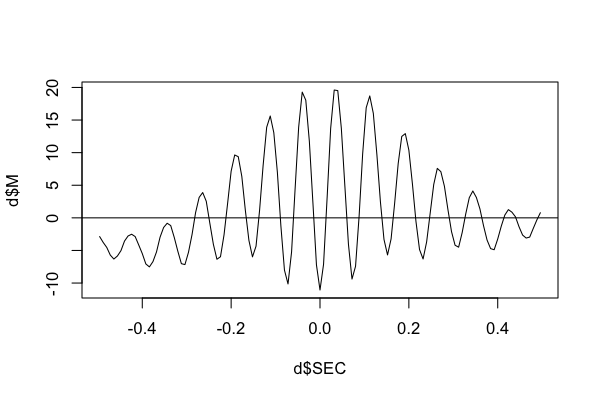
i.e. here we see the characteristic spindle waveform.

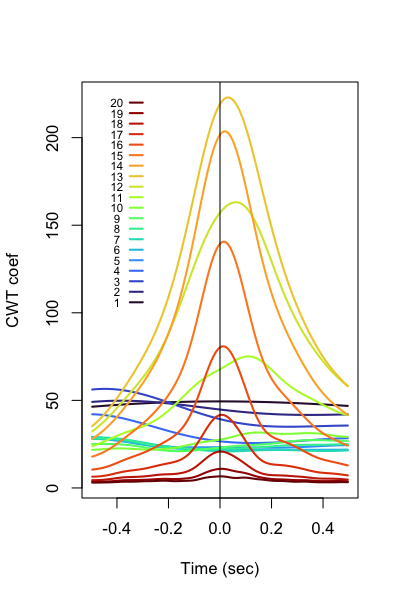
In the second example, we'll create a second set of channels to plot against the 400 spindle peaks. Note, these can be completely arbitrary other channels, but in this instance we'll generate wavelet coefficients (via CWT) for wavelets with central frequency values of 1 Hz to 20 Hz in 1 Hz increments. Then we'll ask TLCOK to plot the time-locked average of each wavelet coefficient, but all time-locked to the fast spindle peaks. i.e. as a proof-of-principle, we'd expect to see sigma-frequency wavelets increase in power in this interval.

luna s.lst -o out.db -s 'MASK ifnot=N2 & RE &
                         CWT sig=EEG fc-inc=1,20,1 cycles=7 &
                         SPINDLES sig=EEG fc=15 cache-peaks=p1 &
                         TLOCK cache=p1 sig=[EEG_cwt_mag_][1:20] w=0.5 '

To plot all signatures in R:

k <- ldb("out.db")
d <- k$TLOCK$CH_SEC_sCH_sF
p20 <- lturbo(20)
plot( d$SEC , d$M , type="n" , xlab = "Time (sec)" , ylab = "CWT coef" )
for (f in 1:20 ) {
 ch <- paste( "EEG_cwt_mag" , f , sep="_" )
 lines( d$SEC[ d$CH == ch ] , d$M[ d$CH == ch ] , lwd=2 , col = p20[f] ) 
}
abline(v=0)
# adhoc legend
for (f in 1:20 ) {
 lines( c(-0.35,-0.3) , c(100+f*6,100+f*6) , lwd=2, col=p20[f] )
 text( -0.4 , 100+f*6 , f , cex=0.7 ) 
}