lunaR plotting functions
Warning
This page is a placeholder and will be completed in due course.
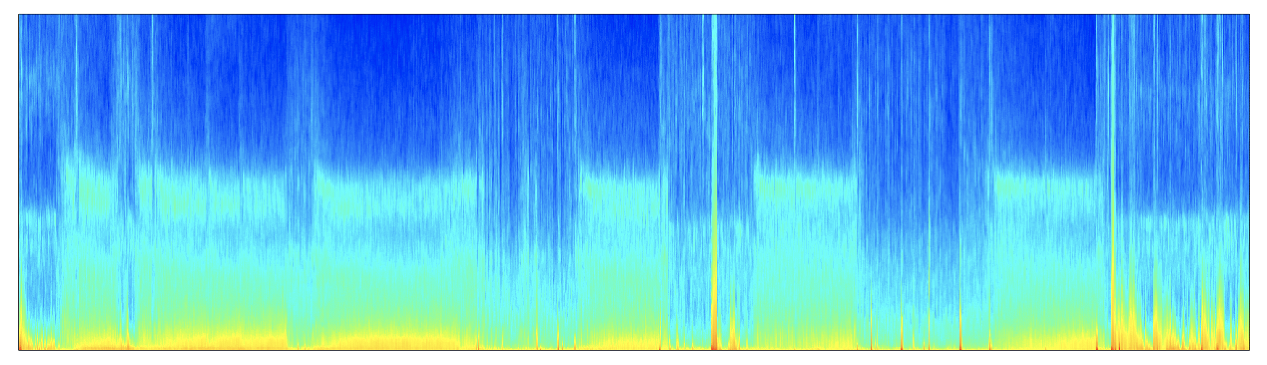
lheatmap()
A simple heatmap
Syntax: lheatmap(x, y , z)
x,yandzare three similarly-sized vectors wherexandydefine a rectangular grid of values, andzis the heat (i.e. plotted value)
Returns: a heatmap image
This simple wrapper will likely need editing to produce high-quality
figures, but it might provide a good starting point. It is designed
to work with data in the format as returned by epoch-spectrum from
PSD and
MTM, for example:
d <- lx( k , "PSD" , "CH" , "E", "F" )
lheatmap( mtm$SEG , mtm$F , mtm$MTM )
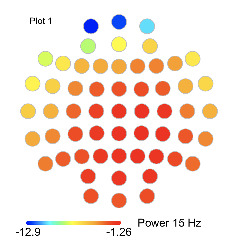
ltopo.heat()
ltopo.heat( psd$CH , psd$PSD , flt = psd$F == 15 , sz = 3 , zlab = "Power 15 Hz", mt = "Plot 1" )
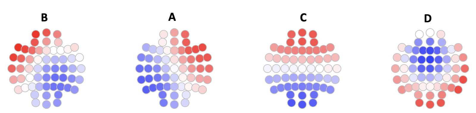
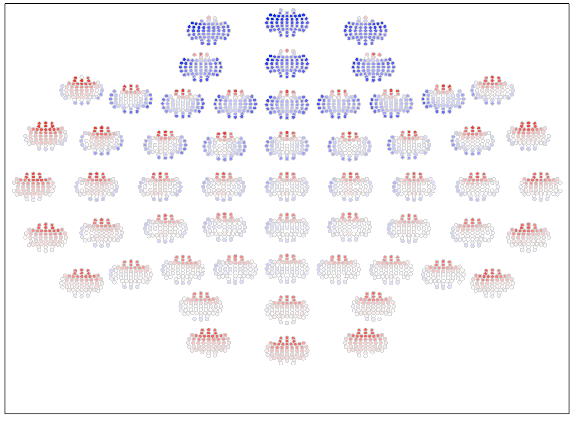
ltopo.rb()
As ltopo.heat() except using a blue (negative) and red (positive) color scale, with 0 as white. This is the
same zeroed=T and with a different color scheme.
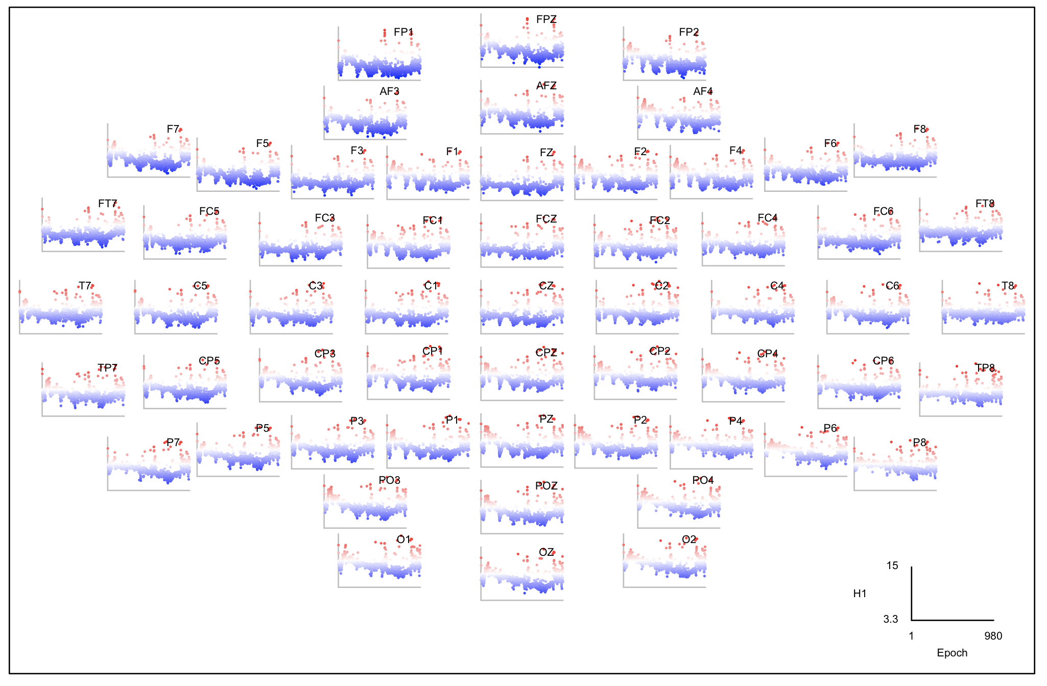
ltopo.xy()
ltopo.xy( c = hj$CH , x = hj$E , y = log( hj$H1 ) , xlab = "Epoch" , ylab = "H1" )
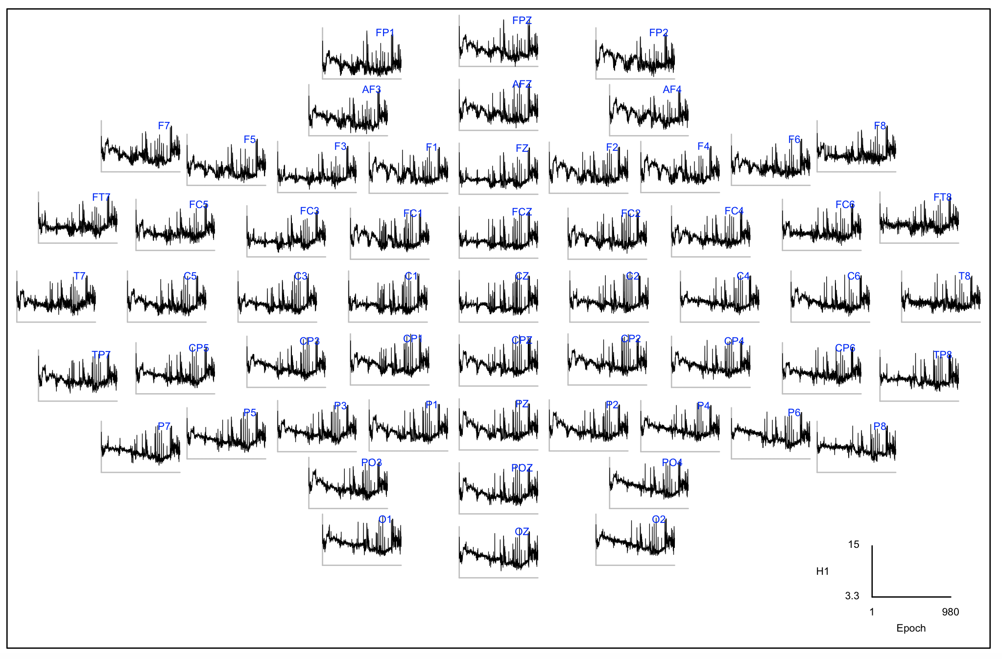
ltopo.xy( c = hj$CH , x = hj$E , y = log( hj$H1 ) , xlab = "Epoch" , ylab = "H1" , z = log( hj$H1 ) , pch=20 , col=rbpal , cex = 0.2 )
ltopo.conn()
ltopo.conn( chs1 = coh$CH1 , chs2 = coh$CH2 , z = coh$COH , flt = coh$B == "DELTA" & coh$COH > 0.8 , w = 3 , zr = c(-1 , 1 ) )
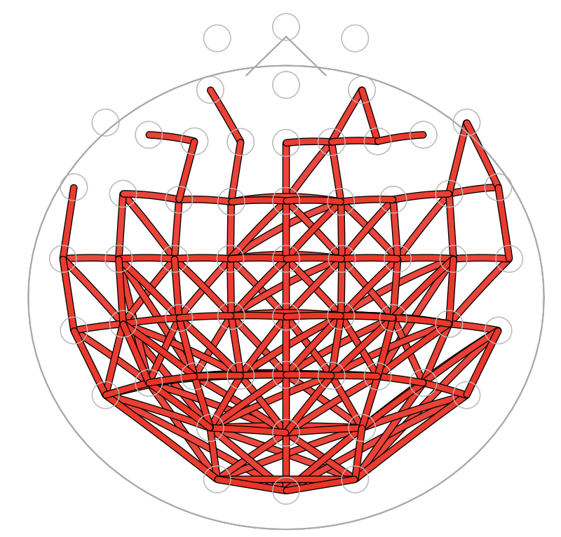
ltopo.conn( chs1 = coh$CH1 , chs2 = coh$CH2 , z = coh$ICOH , flt = coh$B == "SIGMA" & coh$COH > 0.7 , w = 5 , signed = T )
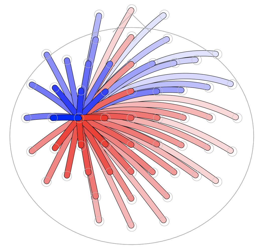
ltopo.dconn()
ltopo.dconn( ch = "C3" , chs1 = coh$CH1 , chs2 = coh$CH2 , z = coh$COH , flt = coh$B == "SIGMA" )
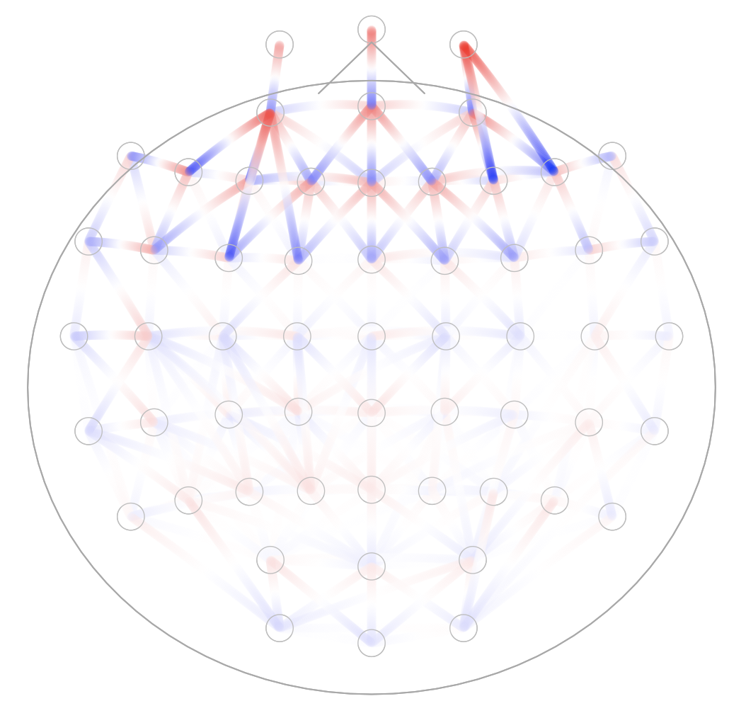
ltopo.topo()
ltopo.topo( c = c( coh$CH1 , coh$CH2 ) , c2 = c( coh$CH2 , coh$CH1 ) , z = c( coh$ICOH , -1 * coh$ICOH ) , f = rep( coh$B == "SIGMA" , 2 ) , sz=0.08, sz2=0.6 )
ldefault.xy()
Default channel co-ordinates for plotting
ldefault.coh.xy()
Default channel co-ordinates for plotting connectivity maps