Association analysis

Efficient sample-level permutation-based association testing

Whereas most Luna commands operate on EDFs in a serial manner, these commands operate at the sample level, on derived metrics (e.g. the output of prior Luna commands, as well as any previously generated arbitrary datasets) and other clinical and demographic covariates. As such, association analyses do not require a sample-list as input and are run via special command-line options.

This page describes two related approaches:

GPA: general pairwise association between two sets of variables (dependent and independent variables)
CPT: specialized variant of the general association model for a single independent variable, featuring cluster-based testing, i.e. pooling across similar metrics, where similarity may be defined by spatial proximity of channels (e.g. Cz and PCz), or by metrics with similar associated frequencies (e.g. 13 Hz and 13.25 Hz), etc. Cluster-based approaches can be more powerful under some conditions.

Both commands use permutation (randomly shuffling rows for some columns of the dataset) to correct for multiple-testing, using the Freedman-Lane approach to handle nuissance variables. Both options also allow for one or more covariates (nuissance variables). The commands primarily differ in whether they allow for clustering of certain types of similar metrics (CPT), or whether they have a slightly more general, flexible specification of many pairwise (non-clustered) tests (GPA). The GPA command should be the default option unless you are specifically interested in cluster-based analyses.

Command	Description
`GPA`	General permutation-based association analysis for one or more sets of metrics
`CPT`	Cluster-based permutation to one or more sets of metrics

GPA

General permutation-based association models

This module comprises two commands:

--gpa-prep which collates one or more text-based input files and generates a compact binary file with all data and meta-data; optionally, specific variables can be included or excluded at this stage, along with some other steps (e.g. variables with completely null/missing values can be dropped). Input data can be listed on the command-line, or they can be described in a special JSON format (described below); the --gpa-prep command also provides an option for automatically generating a base version of the JSON file.
--gpa which reads a binary file created by --gpa-prep, applies various filters and QC steps (e.g. winsorizing, standardizing, optional kNN imputation of missing data, dropping variables with too much missing data, followed by case-wise deletion for missing data), and then applies linear model in a permutation-based framework to perform association analyses whilst controlling multiple testing between one or more dependent (Y) variables and one or more independent predictor (X) variables, allowing for an arbitrary set of covariates (Z)

See this page of the Luna walk-through to see an application of GPA, and the notes below the parameter and output tables for more context.

Parameters

See the documentation below for context on these parameters and outputs tabulated here.

Data preparation with `--gpa-prep`

Primary options:

Option	Example	Description
`inputs`	`a.txt\|grp\|F1`	Specifies one or more input files and key meta-data (groups, factors)
`make-specs`		Create a JSON specification file from the `inputs`
`specs`	`specs.json`	Specifies a JSON file with meta-data on the files, variables and factors, etc
`dat`	`b.1`	Name of the binary data file to be generated

Secondary --gpa-prep options:

Option	Example	Description
`n-req`	10	Require each variable to have at least 10 non-missing values (default: 0)
`n-prop`	0.1	Require each variable to have proportion of at least 0.1 non-missing values (default: 0)
`vars`	`A,B,C`	Only extract these variables from the inputs (default: read all)
`xvars`	`X,Y`	Do not extract these variables from the inputs (default: read all)
`facs`	`F1,F2`	Only read files with these extact factors (default: read all)
`xfacs`	`F3`	Do not read files with these extact factors (default: read all)
`grps`	`grp1,grp2`	Only read files assigned to these groups (default: read all)
`xgrps`	`grp3`	Do not read files assigned to these groups (default: read all)

Data analysis with `--gpa`

Primary analysis options:

Option	Example	Description
`dat`	`b.1`	Read data from this binary file (created by `--gpa-prep`)
`nreps`	10000	Perform association tests, using 10,000 null permutations
`X`	`DIS,QT1`	Set one or more predictor variables
`Z`	`AGE,SEX,WAVE`	Set one or more nuissance variables (covariates)
`Xg`	`preds`	Set predictors based on groups
`Zg`	`covar,demo`	Set covariates based on groups
`n-req`	`10`	Require at least this many non-missing observations to retain a variable (default: 5)
`n-prop`	`0.5`	Require at least this proportion of non-missing observations to retain a variable (default: 0.05)
`knn`	3	Perform kNN missing data imputation (for Y variables only)
`winsor`	0.05	Winsorize all dependent (Y) variables at this proportion
`qc`	`F`	If false, do not perform QC (winsorization and standardization) (default: true)
`adj-all-X`		Adjust for multiple testing across all predictors (otherwise, correction is performed only at the level of each predictor)
`bonf`		Report Bonferroni single-step adjusted p-values
`holm`		Report Holm (1979) step-down adjusted p-values (aka a better Bonferroni)
`fdr`	`F`	Report Benjamini & Hochberg (1995) step-up FDR control (default: `T`, can be set to `F` )
`fdr-by`		Report Benjamini & Yekutieli (2001) step-up FDR control
`adj`		Report all four adjusted p-values
`progress`	`F`	Print progress to the console (default: `T`)

Secondary options: variable selection

Option	Example	Description
`nvars`	`1-10,30-50,100`	Only read these variables from the binary file (default: read all)
`xnvars`	`56,200-300`	Do not read these variables from the binary file (default: read all)
`faclvls`	`CH/CZ\|FZ\|OZ,B/SIGMA\|GAMMA`	Only read variables with these factor-level values (e.g. with channel `CH` Cz, Fz or Oz, and band (`B`) of sigma or gamma)
`xfaclvls`	`B/TOTAL`	Do not read variables with these factor-level values
`lvars`	`PSD_CH_C3_B_SIGMA`	Only read these variables from the binary file based on long variable names (default: read all)
`xlvars`	`PSD_CH_C3_B_SIGMA`	Do not read these variables from the binary file based on long names (default: read all)

Secondary options: selecting subsets of individuals

Option	Example	Description
`ids`	`P1`	Only include individuals (rows) that match this list of `ID` values
`exc-ids`	`P2,P3`	Exclude individuals (rows) that match this list of `ID` values
`subset`	`+DIS`	Include only individuals (rows) that match for the variable `DIS` (any value other than `0`, `NaN` or missing, `NA`); alternatively, if `-DIS` then drop those individuals

Secondary options: analysis parameters

Option	Example	Description
`all-by-all`		Set `X` to the same as all implied `Y` variables, i.e. test all pairwise combinations of a single set of variables

Secondary options: output options

Option	Example	Description
`verbose`		Emit verbose output to the console
`X-factors`		Add X variable factor meta-data to the output (as well as for Y variables)
`progress`	`F`	Show progress of replicates in the log (default=true)
`retain-cols`		Do not drop variables based on invariance (if dumping the file)
`retain-rows`		Do not drop variables based on invariance (if dumping the file)

Secondary options: other summaries

Option	Example	Description
`desc`		Dump a description of the data (its variable/factor structure) to standard output text
`manifest`		Dump the variable manifest (post-filtering & QC) to standard output text
`dump`		Dump the (post-filtered & QC'ed) data file to standard output text
`stats`		Output statistics to the output database
`winsor`	0.01	Winsorize all dependent (_Y) variables
`qc`	`qc=F`	Accepts true/false value for whether to run QC (default: true)
`p`	0.05	Only output tests with pointwise empirical p-value less than this value (default: output all)
`padj`	0.05	Only output tests with adjusted empirical p-value (i.e. corrected for multiple testing) less than this value (default: output all)
`correct-all-X`	`F`	True/false variable, if false perform multiple test correction separately for each `X` variable (default: true, i.e. correct for all tests)

Outputs

Primary outputs (strata: X (IV) x Y (DV)):

Variable	Description
`BASE`	Base variable for the `Y` variable (e.g. `PSD` for `PSD_B_SIGMA_CH_C3` )
`GROUP`	Group to which `Y` belongs
`STRAT`	Key-value pairing for `Y` strata
`N`	Number of non-missing observations
`B`	Beta from linear regression for `Y` variable on `X` predictor
`T`	Corresponding t-statistic
`P`	Uncorrected asymptotic significance value
`P_FDR`	FDR-corrected significance value (q value)
`EMP`	Uncorrected empirical significance value
`EMPADJ`	Family-wise corrected empirical significance value
`P_FDR_BY`	Optional, B&Y FDR-corrected p-value
`P_BONF`	Optional, Bonferroni-corrected p-value
`P_HOLM`	Optional, Holm-corrected p-value

Variable meta-data outputs (strata: X x Y, option: X-factors )

Variable	Description
`GROUP`	Group for the `Y` variable (i.e. based on file inputs )
other factors	e.g. `B` and `CH` for the dependent (`Y`) variables
`XBASE`	(if option `X-factors`) Base variable for the `X` variable
`XGROUP`	(if option `X-factors`) Group for the `X` variable
X plus other factors	(if option `X-factors`) any corresponding factors for the `X` variable

Hint

Avoid factor names that match BASE, GROUP, B, T, P, etc. You can rename factors automatically using the JSON input scheme.

Optional summary statistics (strata: VAR; option: stats)

Variable	Description
`MEAN`	Variable mean
`SD`	Variable SD
`N`	Number of non-missing observations

Usage notes and examples

See the walk-through for a semi-realistic application of GPA to real data. Below, we outline various aspects of GPA:

preparing input data
making/using the JSON specs
variable manifests
kNN missing data imputation
basic QC
individual inclusions/exclusions
variable selection
multiple test correction

Input data

Although GPA can read any standard rectangular (tab-delimited, text-based) data files, it is optimized for reading long-format outputs, as are often generated by Luna, e.g. containing the same metric for multiple channels or frequencies. The --gpa-prep command compiles metrics across one or more files into a single, analysis-ready matrix (each row is one individual and the various features are the columns). Here we give a series of toy examples to illustrate usauge:

All files must have a single header row and a first column named ID (the ID for that observation). Missing data can be encoded as non-numeric values (ideally . or NA). Here we have three individuals, with two variables (A and B) defined for multiple channels (CH). We use the terminology:

CH is a factor
F3 or F4 are the levels of that factor
a particular combination of one or more factors, each with a single associated level, defines a stratum (e.g. CH/C3)

cat d1.txt

ID  CH  A   B
P1  F3  1   1
P1  F4  2   2
P2  F3  3   .
P2  F4  4   .
P3  F3  5   3
P3  F4  6   4

Here we have a second file (d2.txt) containing three new variables (C, D, and E) on the same three individuals:

cat d2.txt

ID  C   D   E
P1  1   2   3
P2  4   NA  5
P3  6   7   8

To read these two files and create a single data matrix using --gpa-prep we can write:

luna --gpa-prep --options dat=b.1 inputs='d1.txt|grp1|CH,d2.txt|grp2' > manifest

  preparing inputs...
  ++ d1.txt: read 3 indivs, 2 base vars --> 4 expanded vars
  ++ d2.txt: read 3 indivs, 3 base vars --> 3 expanded vars

  checking for too much missing data ('retain-cols' to skip; 'verbose' to list dropped vars)
  nothing to check (n-rep and n-prop set to 0)

  writing binary data (3 obs, 7 variables) to b.1
  ...done

The syntax for each input is file|group|factor(s) where the factors are optional (if specified, they should exist as a column in the file, e.g. CH). As above, we see we've generated a matrix b.1 containing 7 variables for 3 individuals. By default, the --gpa-prep commands outputs a manifest to the console, which we redirected here to a file manifest:

cat manifest

NV    VAR       NI   GRP     BASE    CH
0     ID        3    .       ID      .
1     A_CH_F3   3    grp1    A       F3
2     A_CH_F4   3    grp1    A       F4
3     B_CH_F3   2    grp1    B       F3
4     B_CH_F4   2    grp1    B       F4
5     C         3    grp2    C       .
6     D         2    grp2    D       .
7     E         3    grp2    E       .

The manifest effectively describes the columns of the b.1 (binary) data matrix:

NV is the column number (these numbers could be used by lvars etc to select/exclude particular variables
VAR is the generated wide name of the variable, which combines the original (base) variable name with any specific stratum (using _key_value syntax, e.g. _CH_C3)
NI is the number of non-missing individuals for that metric
GRP is the group that metric was assigned to (by the inputs argument)
BASE is the original, base variable name (e.g. to map A_CH_F3 as one instance of A)
CH is a factor with the corresponding level shown for each expanded variable (or . if this is not relevant for a given variable); if other factors exist in the data, these will be listed after (in alphabetical order); obviously, columns six onwards will depend on what factors happen to be present in the input data (if any)

This file is very useful to align to the output of --gpa (as shown in the walkthrough), e.g. to be able to subset tests by a given strata, or to plot by channel, etc, after linking the VAR field in the manifest to the Y field in the output of --gpa, as shown below.

Given a binary file, we can export the contents back as a standard, rectangular tab-delimited file using dump:

luna --gpa --options dat=b.1 dump

  reading binary data from b.1
  reading 7 of 7 vars on 3 indivs
  read 3 individuals and 7 variables from b.1
  selected 0 X vars & 0 Z vars, implying 7 Y vars
  checking for too much missing data ('retain-cols' to skip; 'verbose' to list dropped vars)
  requiring at least n-req=5 non-missing obs (as a proportion, at least n-prop=0.05 non-missing obs)
  dropped 3 vars with too many NA values
  running QC (add 'qc=F' to skip) without winsorization (to set, e.g. 'winsor=0.05')
  retained all observations following case-wise deletion screen
  standardized and winsorized all Y variables

ID A_CH_F3 A_CH_F4       C       E
P1      -1      -1  -1.059  -0.927
P2       0       0  0.1324  -0.132
P3       1       1  0.9272   1.059

As the console log notes, by default this drops variables with missing data, thus we only have 4 of the 7 variables output. By default, GPA requires complete data and will drop rows that don't have missing data; this behavior can be changed with retain-cols (and similarly retain-rows) options. Further, as GPA also by default will attempt to standardize Y variables, we'll also turn this off (by adding qc=F):

luna --gpa --options dat=b.1 dump qc=F retain-cols

ID  A_CH_F3  A_CH_F4  B_CH_F3  B_CH_F4   C   D   E
P1        1        2        1        2   1   2   3
P2        3        4      nan      nan   4 nan   5
P3        5        6        3        4   6   7   8

Now we see the full dataset (with nan indicating missing values, matching the original input data).

Next, we'll extend the dataset by adding three additional files: d3.txt, d4.txt and d5.txt to illustrate various points. The d3 dataset contains a new variable (F) stratified by CH but also SS (e.g. sleep stage) and is present for only two of the three individuals:

cat d3.txt

ID  CH  SS  F
P1  F3  NR  1
P1  F3  R   2
P1  F4  NR  3
P1  F4  R   4
P3  F3  NR  5
P3  F3  R   6
P3  F4  R   7

To illustrate how to specify that metrics have multiple stratifying factors (CH and SS):

luna --gpa-prep --options dat=b.1 \
 inputs='d1.txt|grp1|CH,d2.txt|grp2,d3.txt|grp1|CH|SS'

The generated manifest now has as additional SS column:

NV   VAR           NI   GRP    BASE  CH   SS
0    ID             3   .      ID    .    .
1    A_CH_F3        3   grp1   A     F3   .
2    A_CH_F4        3   grp1   A     F4   .
3    B_CH_F3        2   grp1   B     F3   .
4    B_CH_F4        2   grp1   B     F4   .
5    F_CH_F3_SS_NR  2   grp1   F     F3   NR
6    F_CH_F3_SS_R   2   grp1   F     F3   R
7    F_CH_F4_SS_NR  1   grp1   F     F4   NR
8    F_CH_F4_SS_R   2   grp1   F     F4   R
9    C              3   grp2   C     .    .
10   D              2   grp2   D     .    .
11   E              3   grp2   E     .    .

Next, we'll add the d4 dataset, which contains only A values for a single channel (F3) for two new individuals (P4 and P5):

cat d4.txt

ID  CH  A   
P4  F3  7
P5  F3  8

This demonstrates that the same variable(s) can be distributed across different files for different individuals and still be assembled in the final binary dataset. If the same variable for the same individual is duplicated across files, then only the final value will be used (if the values differ, in which case GPA will issue a warning). Here we have two extra individuals (P4 and P5, neither of wheom are present in the other files). Note that here we use the += syntax to build up a comma-delimited argument:

luna --gpa-prep --options dat=b.1 \
 inputs+='d1.txt|grp1|CH' \
 inputs+='d2.txt|grp2' \
 inputs+='d3.txt|grp1|CH|SS' \
 inputs+='d4.txt|grp1|CH' \
 > manifest

  ++ d1.txt: read 3 indivs, 2 base vars --> 4 expanded vars
  ++ d2.txt: read 3 indivs, 3 base vars --> 3 expanded vars
  ++ d3.txt: read 2 indivs, 1 base vars --> 4 expanded vars
  ++ d4.txt: read 2 indivs, 1 base vars --> 1 expanded vars

  writing binary data (5 obs, 11 variables) to b.1
  ...done

That is, writing

v=a
v+=b
v+=c

is the same as writing v=a,b,c. Note that it is still necessary to quote the arguments (to stop the | character being interpreted by the shell) and to use \ as the last character on each line to denote a multi-line statement.

To check these inputs were processed correctly, we can dump the file again:

luna --gpa --options dat=b.1 dump qc=F retain-cols

ID A_CH_F3 A_CH_F4 B_CH_F3 B_CH_F4 F_CH_F3_SS_NR F_CH_F3_SS_R F_CH_F4_SS_NR F_CH_F4_SS_R    C    D    E
P1       1       2       1       2             1            2             3            4    1    2    3
P2       3       4     nan     nan           nan          nan           nan          nan    4  nan    5
P3       5       6       3       4             5            6           nan            7    6    7    8
P4       7     nan     nan     nan           nan          nan           nan          nan  nan  nan  nan
P5       8     nan     nan     nan           nan          nan           nan          nan  nan  nan  nan

That is, P4 and P5 have a lot of missing data, as this they only had a single variable specified (A for CH = F3).

Finally, we'll add the d5 dataset, which contains clinical/demographic information (disease status and sex) for all individuals; note that sex is encoded as a string (M/F) whereas GPA expects numeric inputs, and includes a missing value (?):

cat d5.txt

ID  SEX DIS
P1  F   T
P2  F   T
P3  M   F
P4  M   F
P5  ?   T

luna --gpa-prep --options dat=b.1 \
 inputs+='d1.txt|grp1|CH' \
 inputs+='d2.txt|grp2' \
 inputs+='d3.txt|grp1|CH|SS' \
 inputs+='d4.txt|grp1|CH' \
 inputs+='d5.txt|demo' \
 > manifest

When we dump the dataset (here just for DIS and SEX) we'll see that the non-numeric inputs weren't rendered as expected:

luna --gpa --options dat=b.1 dump qc=F  retain-cols vars=DIS,SEX

ID    DIS   SEX
P1    1     0
P2    1     0
P3    0     nan
P4    0     nan
P5    1     nan

Although GPA expects only numeric data as inputs, it provides two "convenience" functions, whereby any values starting with the character Y/N or T/F are mapped to 0/1 respectively (insensitive to case). Here, F is intended to stand for female rather than false, but it is interpreted as such; likewise, M is set to missing (as is ?). Thus the output above.

The bottom line is that you should ensure that string values are transformed prior to GPA input unless you are sure that only the simple exceptions (true/false and yes/no) exist in the file. GPA provides a mechanism for doing this explicitly, but only when using the second "JSON" mode of specifying inputs, which uses the form specs=file.json rather than inputs=....

First, we'll generate a base JSON file that matches what we've already specified via the inputs statement, using the make-specs option of --gpa-prep. Now, instead of making a binary data file and outputting the variable manifest, it will output (to standard output) only the file specification in JSON format:

luna --gpa-prep --options make-specs \
 inputs+='d1.txt|grp1|CH' \
 inputs+='d2.txt|grp2' \
 inputs+='d3.txt|grp1|CH|SS' \
 inputs+='d4.txt|grp1|CH' \
 inputs+='d5.txt|demo' \
 > specs.json

  writing .json specification (from inputs) to standard output
  found 2 variables and 1 factors from d1.txt
  found 3 variables and 0 factors from d2.txt
  found 1 variables and 2 factors from d3.txt
  found 1 variables and 1 factors from d4.txt
  found 2 variables and 0 factors from d5.txt

This JSON specification file now contains the same information as encoded in the inputs line. It can be convenient to use this form however, and a) it can be modified to provide additional functionality, as we'll see below, including restricting inputs to subsets of variables/values and transforming values, and b) these files can be re-used across different cohorts (i.e. if they are being applied to the same set of metrics).

cat specs.json

{
  "inputs": [
    {
      "group": "grp1",
      "file": "d1.txt",
      "facs": [ "CH" ],
      "vars": [ "A", "B" ]
    },
    {
      "group": "grp2",
      "file": "d2.txt",
      "vars": [ "C", "D", "E" ]
    },
    {
      "group": "grp1",
      "file": "d3.txt",
      "facs": [ "CH", "SS" ],
      "vars": [ "F" ]
    },
    {
      "group": "grp1",
      "file": "d4.txt",
      "facs": [ "CH" ],
      "vars": [ "A" ]
    },
    {
      "group": "demo",
      "file": "d5.txt",
      "vars": [ "SEX", "DIS" ]
    }
  ]
}

We could have generated this text file by hand, or using other tools, but make-specs os provided as a convenience function, as writing JSON by hand can be tedious. Given a JSON specification file (that can be called anything, but we recommend a .json extension) we could create the binary file as follows:

luna --gpa-prep --options dat=b.1 specs=specs.json > manifest

  parsing specs.json
  reading file specifications ('inputs') for 5 files:
   d1.txt ( group = grp1 ): 
    expecting 1 factors, extracting 2 var(s)
   d2.txt ( group = grp2 ): 
    expecting 0 factors, extracting 3 var(s)
   d3.txt ( group = grp1 ): 
    expecting 2 factors, extracting 1 var(s)
   d4.txt ( group = grp1 ): 
    expecting 1 factors, extracting 1 var(s)
   d5.txt ( group = demo ): 
    expecting 0 factors, extracting 2 var(s)

  preparing inputs...
  ++ d1.txt: read 3 indivs, 2 base vars --> 4 expanded vars
  ++ d2.txt: read 3 indivs, 3 base vars --> 3 expanded vars
  ++ d3.txt: read 2 indivs, 1 base vars --> 4 expanded vars
  ++ d4.txt: read 2 indivs, 1 base vars --> 1 expanded vars
  ++ d5.txt: read 5 indivs, 2 base vars --> 2 expanded vars

  checking for too much missing data ('retain-cols' to skip; 'verbose' to list dropped vars)
  nothing to check (n-rep and n-prop set to 0)

  writing binary data (5 obs, 13 variables) to b.1
  ...done

That is, we've achieved the same results as above, just using the JSON method to specify what and where these data live. As noted, this allows us to make additional qualifications:

renaming variables or factors
adding fixed factors to a file
mapping text values to numeric values
excluding certain variables, or only retaining certain variables prior to making the binary file

We'll first consider mapping text to numeric values, as motivated by the handling of SEX above, using a text editor to modify the part of the JSON that specifies the d5.txt inputs, i.e. originally:

{
  "group": "demo",
  "file": "d5.txt",
  "vars": [ "SEX", "DIS" ],
}

We'll make two changes:

First, we'll rename the variable SEX to MALE, to clarify the meaning of 0/1 encoding (i.e. 1 will indicate a male). We do this by replacing the single string value "SEX" with the key-value object {"SEX": "MALE"}. This tells GPA to replace all variable name instances of SEX with MALE. This aliasing of input variables can be applied to any of the listed variables.
Second, we'll add an extra "mappings" entry to this file object. (Note that we also need to put an extra comma at the end of the line starting "vars" too, or else we'll get a JSON syntax error.) The mappings entry take an array ([ ]) where each entry is an object in the form { var: { str: num } }, meaning that the string str should be swapped to the number num for variable var. As we've already specified an alias for SEX, we should use that term here (i.e. the variable will be called MALE when processing the file).

The final entry should read as follows:

{
  "group": "demo",
  "file": "d5.txt",
  "vars": [ {"SEX":"MALE"}, "DIS" ],
  "mappings": [ {"MALE": { "M":1 } } , {"MALE": {"F": 0} } ]
}

If we remake the binary dataset with the modified JSON specs:

luna --gpa-prep --options dat=b.1 specs=specs.json > manifest

We now see the correct information listed (note that P5 had missing data in the original):

luna --gpa --options dat=b.1 dump qc=F retain-cols vars=DIS,MALE

ID    DIS    MALE
P1    1      0
P2    1      0
P3    0      1
P4    0      1
P5    1      nan

To give a further example of modifying the JSON, it can sometimes be convenient to add fixed factors to a file: for example, if results from different sleep stages are in different files, but don't themselves contain additional variables that would distinguish them after merging. Consider two other files (separate from the examples given above):

cat nrem-metrics.txt

ID       M1
I001  -1.07
I002   2.11
I003   4.34

cat rem-metrics.txt

ID       M1
I001   3.21
I002  -0.22
I003   3.17

Here we have the same variable (M1) defined in two sleep stages, but that distinction is only implicit by the file names, not the variable names. If we were to read both files as is:

luna --gpa-prep --options dat=b.1 'inputs=nrem-metrics.txt|nrem,rem-metrics.txt|rem'

  preparing inputs...
  ++ nrem-metrics.txt: read 3 indivs, 1 base vars --> 1 expanded vars
  ++ rem-metrics.txt: read 3 indivs, 1 base vars --> 1 expanded vars

  writing binary data (3 obs, 1 variables) to b.1
  ...done

We see that only a single M1 metric is generated:

NV    VAR    NI    GRP    BASE
0      ID     3      .      ID
1      M1     3   nrem      M1

You'll see the log reported warnings:

  *** warning *** repeated instances of M1 for I001 (-1.07 and 3.21)
  *** warning *** repeated instances of M1 for I002 (2.11 and -0.22)
  *** warning *** repeated instances of M1 for I003 (4.34 and 3.17)

which means the data will not be correctly read in and that it is therefore necessary to disambiguate these metrics. (Note that the group variable doesn't explcitily separate out these two variables: groups are only used as a shorthand to refer to sets of variables, e.g. to include or exclude from analyses).

To rectify this issue, we could explicitly add the relevant stratifiers to the data files, for example:

cat nrem-metrics.txt

ID       M1    SS
I001  -1.07    NR
I002   2.11    NR
I003   4.34    NR

and likewise for the REM data. As an alternative, that may often be easier if dealing with multiple large files, we can achieve the same effect by modifying the JSON specification file describing these data. If we first generate it as above:

luna --gpa-prep --options make-specs \
  'inputs=nrem-metrics.txt|nrem,rem-metrics.txt|rem' > specs2.json

cat specs2.json

{
  "inputs": [
    {
      "group": "nrem",
      "file": "nrem-metrics.txt",
      "vars": [ "M1" ]
    },
    {
      "group": "rem",
      "file": "rem-metrics.txt",
      "vars": [ "M1" ]
    }
  ]
}

We'll now add "fixed" entries to these files, which will effectively add that factor/level pair (e.g. values of NR for a variable called SS) for every row in that file:

{
  "inputs": [
    {
      "group": "nrem",
      "file": "nrem-metrics.txt",
      "vars": [ "M1" ],
      "fixed": [ { "SS": "NR" } ] 
    },
    {
      "group": "rem",
      "file": "rem-metrics.txt",
      "vars": [ "M1" ],
      "fixed": [ { "SS": "R" } ]
    }
  ]
}

If we now use this appropriately modified file to read the data, it will correctly keep the NREM and REM data separate:

luna --gpa-prep --options dat=b.1 specs=specs2.json

  reading file specifications ('inputs') for 2 files:
   nrem-metrics.txt ( group = nrem ): 
    expecting 0 factors and 1 fixed factors, extracting 1 var(s)
   rem-metrics.txt ( group = rem ): 
    expecting 0 factors and 1 fixed factors, extracting 1 var(s)

The manifest now reflects both variables with the correct SS tags:

NV      VAR   NI   GRP   BASE   SS
0        ID    3     .     ID    .
1  M1_SS_NR    3  nrem     M1   NR
2   M1_SS_R    3   rem     M1    R

Now, when dumping the b.1 binary file using the same command as above we see the correct values:

ID    M1_SS_NR  M1_SS_R
I001     -1.07     3.21
I002      2.11    -0.22
I003      4.34     3.17

To summarize some key concepts for data input:

all input files must contain ID as the first column and be tab-delimited with a fixed number of columns; otherwise, the order of rows or columns across files does not matter
variables are ordered in the manifest (and final data file) by group (alphabetically) and then by base variable name
different factor/level combinations are listed in the same order as they are first encountered in the input files
the group labels are provided only to provide convenient ways to group variables in the manifest, and also to select/exclude whole sets of variables
more than one file can be assigned to a group; if there is no relevant grouping among variables, you can set all groups to an arbitrary string (e.g. all)
the numbers in the manifest (NV) correspond to the number system that can be used to subsequently select variables for analysis (using nvars and xnvars)
all association tests require full data; options to retain columns or rows with missing (or invariant) data (i.e. qc=F, retain-cols and retain-rows) are only applicable if using --gpa to dump a file (rather than running association models); one can potentially impute missing data via kNN imputation as described below

JSON specs

The JSON specs should have the following minimal form with one or more files:

{
  "inputs": [ {x}, {x}, {x} ] 
}

where each {x} describes one file. The file specification should be of the minimal form:

{
    "file": "results/metrics.txt",
    "group": "eeg"
}

Other file attributes include:

"vars" - an array of variables to read (if omitted, all non-factor variables will be read)
"xvars" - an array of variables to exclude
"facs" - an array of factors (expected to be present in the header of the file); these fields will not be read of variables, but rather as stratifying factors, e.g. [ "CH", "F" ]
"fixed" - as above, specifying one or more fixed factors for that file (i.e. setting for all rows, assuming the file doesn't already contain that field)
"mappings" - as above, instructions to recode strings to numeric values for a given variable

Manifests

The basic --gpa-prep outputs a variable manifest.

Alternatively, given a binary file, you can retrieve the matching manifest as follows (here saving it to a text file called manifest):

luna --gpa --options dat=b.1 manifest > manifest

The format of the manifest is described in the section above.

kNN imputation

For applications with many dependent variables, but low or modest rates of missing data, one can request kNN imputation. Adding the, e.g., knn=5 option to --gpa will attempt to impute missing missing data based on k nearest neighbors (i.e. here k = 5). This is performed only for the dependent (Y) variables, not for any predictors or covariates; further, only dependent variables are used in determining the individuals who are "similar" to a given individual (and so this procedure should not unduly introduce spurious relationships between predictor and outcome variables).

Inclusions/exclusions

You can limit which individuals are read from a binary matrix file, e.g. to perform analyses on only subsets of individuals, with either inc-ids, exc-ids or subset options to --gpa.

It is often useful to combine inc-ids or exc-ids options with the @{include} directive, which reads a list of values from a text file (named include in this example) assuming one-value-per-line. It creates a matching comma-delimited string: e.g. if exclude.txt is:

p0022
p0132
p0288

then

luna --gpa -o out.db \
     --options dat=b.1 nreps=10000 X=DIS inc-ids=@{exclude.txt}

is the same as writing out:

luna --gpa -o out.db \
     --options dat=b.1 nreps=10000 X=DIS inc-ids=p0022,p0132,p0288

Instead of using inc-ids or exc-ids to include or explicitly exclude certain individuals, the subset option can include or exclude on the basis of variables values. For example, if a variable MALE exists coded 0/1, then subset=MALE (or subset=+MALE) will include only people with non-null values for MALE (i.e. not 0 but also not missing). In contrast, subset=-MALE would exclude people with non-null values for MALE. You can combine options conditions, e.g. subset=MALE,-GROUP2 etc. The subset option always requires a simple true/false (encoded 0/1) variable.

Variable selection

Variable selection from a binary dataset operates on two levels:

which variables are extracted from the dataset and brought into memory
of the variables brought into memory, whether they are assigned to be dependent variables (Y), independent variables (X) or covariates (Z)

We'll illustrate some of these steps with the toy dataset above (as above, adding options to ensure that non variables are dropped due to missing data in this toy example):

luna --gpa --options dat=b.1 qc=F retain-cols desc

  reading binary data from b.1
  reading 13 of 13 vars on 5 indivs
  read 5 individuals and 13 variables from b.1
  selected 0 X vars & 0 Z vars, implying 13 Y vars

As the console log notes, there are 13 variables in all, all of which are read in. In the absence of specifying explicit predictor/covariate measures, all variables are (by default) assumed to be outcomes. (Note: association analyses will only be performed if at least one dependent and at least one predictor variable have been specified.)

The desc option gives the following information about the dataset:

  Summary for (the selected subset of) b.1

  # individuals (rows)  = 5
  # variables (columns) = 13

  ------------------------------------------------------------
  8 base variable(s):

    A --> 2 expanded variable(s)
    B --> 2 expanded variable(s)
    C --> 1 expanded variable(s)
    D --> 1 expanded variable(s)
    DIS --> 1 expanded variable(s)
    E --> 1 expanded variable(s)
    F --> 4 expanded variable(s)
    MALE --> 1 expanded variable(s)

  ------------------------------------------------------------
  3 variable groups:

    demo:
         2 base variable(s) ( DIS MALE )
         2 expanded variable(s)
         no stratifying factors

    grp1:
         3 base variable(s) ( A B F )
         8 expanded variable(s)
         2 unique factors:
           CH -> 2 level(s):
             CH = F3 --> 4 expanded variable(s)
             CH = F4 --> 4 expanded variable(s)
           SS -> 2 level(s):
             SS = NR --> 2 expanded variable(s)
             SS = R --> 2 expanded variable(s)

    grp2:
         3 base variable(s) ( C D E )
         3 expanded variable(s)
         no stratifying factors

  ------------------------------------------------------------

If we instead add the manifest option instead of desc, we see these 13 variables:

NV   VAR             NI   GRP     BASE   CH    SS
0    ID              5    .       ID     .     .
1    DIS             5    demo    DIS    .     .
2    MALE            4    demo    MALE   .     .
3    A_CH_F3         5    grp1    A      F3    .
4    A_CH_F4         3    grp1    A      F4    .
5    B_CH_F3         2    grp1    B      F3    .
6    B_CH_F4         2    grp1    B      F4    .
7    F_CH_F3_SS_NR   2    grp1    F      F3    NR
8    F_CH_F3_SS_R    2    grp1    F      F3    R
9    F_CH_F4_SS_NR   1    grp1    F      F4    NR
10   F_CH_F4_SS_R    2    grp1    F      F4    R
11   C               3    grp2    C      .     .
12   D               2    grp2    D      .     .
13   E               3    grp2    E      .     .

There are various options to restrict which variables are extracted:

vars selects variables based on the base variable name (BASE)
lvars selects variables based on the expanded variable name (VAR)
nvars selects variables based on the variable number (NV)
grps selects variables based on the group (GRP)
facs selects variables based on the presence of certain factors (e.g. having a CH factor)
faclvlsselects variables based on matching certain strata (e.g. having F3 for CH)

Each of these inclusion options has a complementary exclusion term: xvars, xlvars, xnvars, xgrps, xfacs and xfaclvls.

If multiple types of inclusion option are specified, they combine using AND logic. If multiple exclusion options are specified they combine using OR logic.

Some examples (excluding ID in each case, which will always be present in the manifest / internally), showing in each case what would be the resulting manifest if this option was added.

Include variables from only A or C bases:

vars=A,C

NV  VAR      NI   GRP   BASE   CH
1   A_CH_F3  5   grp1      A   F3
2   A_CH_F4  3   grp1      A   F4
3   C        3   grp2      C    .

Include variables from grp2 or demo groups:

grps=grp2,demo

NV  VAR   NI    GRP   BASE
1   DIS    5   demo    DIS
2   MALE   4   demo   MALE
3   C      3   grp2      C
4   D      2   grp2      D
5   E      3   grp2      E

Combine the previous two options (i.e. which here uses AND logic), i.e. giving the intersection of matches: ( in group demo OR grp2 ) AND ( of base variable A OR C ):

vars=A,C grps=grp2,demo

NV   VAR   NI   GRP    BASE
1    C     3    grp2   C

To select based on a long variable long:

lvars=F_CH_F3_SS_NR,F_CH_F4_SS_R

NV   VAR            NI  GRP    BASE   CH   SS
1    F_CH_F3_SS_NR  2   grp1   F      F3   NR
2    F_CH_F4_SS_R   2   grp1   F      F4   R

To select based on variable number:

nvars=3,6-8

NV   VAR            NI   GRP     BASE   CH    SS
1    A_CH_F3        5    grp1    A      F3    .
2    B_CH_F4        2    grp1    B      F4    .
3    F_CH_F3_SS_NR  2    grp1    F      F3    NR
4    F_CH_F3_SS_R   2    grp1    F      F3    R

(Note: NV in the manifest always start from 1 and identify the slot for that variable in the subsetted dataset, not the original.)

To select variables stratifed by CH only:

facs=CH

NV   VAR       NI   GRP    BASE   CH
1    A_CH_F3   5    grp1   A      F3
2    A_CH_F4   3    grp1   A      F4
3    B_CH_F3   2    grp1   B      F3
4    B_CH_F4   2    grp1   B      F4

To select variables stratified by CH and SS:

facs=CH,SS

NV   VAR             NI  GRP    BASE   CH   SS
1    F_CH_F3_SS_NR   2   grp1   F      F3   NR
2    F_CH_F3_SS_R    2   grp1   F      F3   R
3    F_CH_F4_SS_NR   1   grp1   F      F4   NR
4    F_CH_F4_SS_R    2   grp1   F      F4   R

That is, for facs (and xfacs) unlike some of the earlier options (e.g. vars and grps, etc) the multiple factors specified here are taken to define a single set of strata (i.e. with the terms combining with AND logic).

Finally, to select based on levels of particular factors, e.g. only F3 values for CH:

faclvls=CH/F3

NV  VAR            NI  GRP    BASE   CH   SS
1   A_CH_F3        5   grp1   A      F3   .
2   B_CH_F3        2   grp1   B      F3   .
3   F_CH_F3_SS_NR  2   grp1   F      F3   NR
4   F_CH_F3_SS_R   2   grp1   F      F3   R

That is, this selects only variables that have the CH factor and the level F3. You also combine multiple levels for a given factor (delimiting with |) as well as multiple factors: e.g. this selects variables with a CH factor that is F3, or those with an SS factor that is NR or R:

faclvls="CH/F3|F4,SS/NR"

NV   VAR             NI   GRP    BASE   CH    SS
1    A_CH_F3         5    grp1   A      F3    .
2    A_CH_F4         3    grp1   A      F4    .
3    B_CH_F3         2    grp1   B      F3    .
4    B_CH_F4         2    grp1   B      F4    .
5    F_CH_F3_SS_NR   2    grp1   F      F3    NR
6    F_CH_F4_SS_NR   1    grp1   F      F4    NR

In practice, working with real outputs, one might want to combine options, e.g. to look at slow spindle (F set to 11 Hz) density (DENS) for all channels during N3 sleep:

vars=DENS faclvls=SS/N3,F/11

After loading some number of variables from the binary dataset, as in the previous examples, GPA still has to know how to assign them for association testing: are they dependent variables (Y), independent variables (X) or covariates (Z)? (Of course, statistically there is no distinction between independent and covariates when fitting the model. Rather, the X versus Z distinction impacts:

which term the output is given for (i.e. betas and significance values from the multiple regression model)
if there are multiple X, they are iterated over selecting one-at-a-time (i.e. fitting a different model for each)
if there are multiple Z, they are all entered simultaneously in every model (for every pair of X and Y variables)

We can control which variables are which by the X, Z and Y commands (and the group-level analogs Xg, Zg and Yg). Specifying some predictor variables tells GPA to fit association models to the data. By default, all selected variables that aren't set as predictors or covariates are assumed to be dependent variables, thus the message:

  read 5 individuals and 5 variables from b.1
  selected 0 X vars & 0 Z vars, implying 5 Y vars

The X, Y and Z options take base variable names, similar to vars; the Xg, Yg and Zg options take group names, similar to grps.

Here we select two predictor variables (D and E) and two covariates (DIS and MALE) specified by the group label demo:

X=D,E Zg=demo

  read 5 individuals and 13 variables from b.1
  selected 2 X vars & 2 Z vars, implying 9 Y vars

Importantly, if specifying variables via X and/or Z, one doesn't need to put them explicitly on the vars inclusion list. That is, one doesn't need to write:

vars=D,E X=D,E grps=demo Zg=demo

(This is important, as as the presence of any vars group will imply that only those variables are extracted from the binary file, i.e. this would exclude the 9 variables that (by default) are set to be the dependents.)

Here, all other (i.e. 13 - 4 = 9) variables are then assumed to be dependent variables. As there are two X variables, this implies a total of 19 tests, which we'd see in the console:

  18 total tests specified

(Note: in the toy datasets above, because of the large amount of missing data, there would not be 18 tests - here we assume we have complete non-missing data for all values to make the description of using X/Z options clearer.)

The outputs would have the form (with each term being from a model with DIS and MALE covariates included):

destrat out.db +GPA -r X Y -v BASE STRAT

ID  X   Y              BASE   STRAT
.   D   A_CH_F3        A      CH=F3
.   D   A_CH_F4        A      CH=F4
.   D   B_CH_F3        B      CH=F3
.   D   B_CH_F4        B      CH=F4
.   D   F_CH_F3_SS_NR  F      CH=F3;SS=NR     
.   D   F_CH_F3_SS_R   F      CH=F3;SS=R     
.   D   F_CH_F4_SS_NR  F      CH=F4;SS=NR     
.   D   F_CH_F4_SS_R   F      CH=F4;SS=R     
.   D   C              C      NA         
.   E   A_CH_F3        A      CH=F3     
.   E   A_CH_F4        A      CH=F4     
.   E   B_CH_F3        B      CH=F3     
.   E   B_CH_F4        B      CH=F4     
.   E   F_CH_F3_SS_NR  F      CH=F3;SS=NR     
.   E   F_CH_F3_SS_R   F      CH=F3;SS=R     
.   E   F_CH_F4_SS_NR  F      CH=F4;SS=NR     
.   E   F_CH_F4_SS_R   F      CH=F4;SS=R     
.   E   C              C      NA

For example, to only these for the F3 channel:

X=D,E Zg=demo faclvls=CH/F3

  reading 8 of 13 vars on 5 indivs
  read 5 individuals and 8 variables from b.1
  selected 2 X vars & 2 Z vars, implying 4 Y vars

ID  X   Y              BASE   STRAT
.   D   A_CH_F3        A      CH=F3
.   D   B_CH_F3        B      CH=F3
.   D   F_CH_F3_SS_NR  F      CH=F3;SS=NR
.   D   F_CH_F3_SS_R   F      CH=F3;SS=R
.   E   A_CH_F3        A      CH=F3
.   E   B_CH_F3        B      CH=F3
.   E   F_CH_F3_SS_NR  F      CH=F3;SS=NR
.   E   F_CH_F3_SS_R   F      CH=F3;SS=R

Alternatively, to exclude A from the set of things tested:

X=D,E Zg=demo xvars=A

  reading 11 of 13 vars on 5 indivs
  read 5 individuals and 11 variables from b.1
  selected 2 X vars & 2 Z vars, implying 7 Y vars

ID  X   Y              BASE   STRAT
.   D   B_CH_F3        B      CH=F3
.   D   B_CH_F4        B      CH=F4    
.   D   F_CH_F3_SS_NR  F      CH=F3;SS=NR    
.   D   F_CH_F3_SS_R   F      CH=F3;SS=R    
.   D   F_CH_F4_SS_NR  F      CH=F4;SS=NR    
.   D   F_CH_F4_SS_R   F      CH=F4;SS=R    
.   D   C              C      NA        
.   E   B_CH_F3        B      CH=F3    
.   E   B_CH_F4        B      CH=F4    
.   E   F_CH_F3_SS_NR  F      CH=F3;SS=NR    
.   E   F_CH_F3_SS_R   F      CH=F3;SS=R    
.   E   F_CH_F4_SS_NR  F      CH=F4;SS=NR    
.   E   F_CH_F4_SS_R   F      CH=F4;SS=R    
.   E   C              C      NA

Finally, to only include F and C variables in the set of dependents:

Zg=demo X=D,E force-zeros vars=F,C

  reading 9 of 13 vars on 5 indivs
  read 5 individuals and 9 variables from b.1
  selected 2 X vars & 2 Z vars, implying 5 Y vars

ID  X   Y              BASE  STRAT
.   D   F_CH_F3_SS_NR  F     CH=F3;SS=NR
.   D   F_CH_F3_SS_R   F     CH=F3;SS=R
.   D   F_CH_F4_SS_NR  F     CH=F4;SS=NR
.   D   F_CH_F4_SS_R   F     CH=F4;SS=R
.   D   C              C     NA
.   E   F_CH_F3_SS_NR  F     CH=F3;SS=NR
.   E   F_CH_F3_SS_R   F     CH=F3;SS=R
.   E   F_CH_F4_SS_NR  F     CH=F4;SS=NR
.   E   F_CH_F4_SS_R   F     CH=F4;SS=R
.   E   C              C     NA

Note that you can restrict which variables are dependent variables with the usual vars/grps/etc as above, or by explicitly specifying the dependent variables via Y (or Yg), rather than have them be whatever is left over after specifying X and Z.

Multiple test correction

In the above examples, with at least 1 X and 1 Y variable specified, GPA will fit a series of linear models. By default, each output row will have statistics for that particular X/Y variable pair: beta (B), t-statistic (T) and p-value (P).

If there are multiple tests, then corrected p-values will also be added. By default, GPA applies Benjamini & Hochberg (1995) to control the false-discovery rate (FDR). These FDR-corrected p-values are reported as P_FDR. Other corrections can be requested:

bonf : Bonferroni single-step adjusted p-values (P_BONF)
holm : Holm (1979) step-down adjusted p-values (P_HOLM)
bonf-by : Benjamini & Yekutieli (2001) (P_FDR_BY )

As well as the corrected asymptotic p-values, GPA can provide empirical p-values that control the family-wide type I error rate allowing for correlation between tests. This is achieved by adding the option nreps=5000 where nreps is set to some sufficiently high number (in practice, at least 1000 to give reasonable corrected p-values around the 0.05 region: more replicates will lead to more stable empirical p-values). The smallest possible empirical p-value is 1/(1+nreps). This option will add the output fields EMP (pointwise empirical p-value) and EMPADJ (multple-test corrected empirical p-value, based on comparing the absolute t-statistic to the maximum of all absolute t-statistics over tests for each null replicate). This uses the Freedman-Lane procedure to appropriately allow for covariates whilst performing permutation.

By default, whether using FDR or empirical approaches, GPA corrects all Y (DV) tests for a given X (IV) variable. This behavior can be changed by adding the option adj-all-X: now GPA will correct over all tests performed (i.e. this is more conservative).

See the Luna walkthrough for examples of applying and working with large GPA outputs - e.g. linking with the manifest information to generate topoplots of results, as well as producing summaries (e.g. number of 'hits' per channel, or metric type, etc).

CPT

Cluster-based permutation analysis

This command fits a set of linear models, using a permutation-based approach that allows for covariates, to generate pointwise empirical significance values, as well as family-wise corrected empirical p-values.

It additionally employs a simple clustering heuristic to find groups of adjacent predictors, and to evaluate the evidence for association over these clusters, based on the sum of test statistics. This command is set up to define clusters with respect to three types of adjacency:

by frequency (e.g. power for 4.5 Hz and 5.0 Hz might be tested jointly)
by spatial location (e.g. CZ and C1 might be considered nearby, and so tested jointly)
by pairs of channels (e.g. for connectivity measures, the pair C3-F1 might be considered adjacent to CZ-FZ)
by time (e.g. for peri-event data)

These stratifiers are automatically determined by the presence of F, CH or CH1 and CH2 or T columns in the dependent variable files.

The idea behind cluster-based analyses non-parametric analysis (outlined here) is that power might be increased by searching for more modest effects that span "similar" predictors, with respect to topography or frequency.

This command can accept multiple types of DV in the same analysis: e.g. spindle density (DENS) as well as amplitude (AMP). With respect to multiple test correction (the PC and cluster-based empirical p-values below), this analysis will correct for both sets of values (accounting for any correlation between them). However, clustering only happens within a particular class of variable. That is, if each mesaure is present for 64 EEG channels, clusters of topographically adjacent channels may be formed for DENS, and separate clusters may be formed for AMP, but no cluster would contain both DENS and AMP measures (i.e. because there is no general way to specify the adjacency of different classes of variable).

The approach to permutation with nuissance variables is the Freedman-Lane method and follows an implementation described here.

Hint

For correctly-formated inputs, the CPT command can be used to analyse any types of numeric inputs, whether they come from prior Luna commands or not.

Parameters

Primary parameters to specify the data and any outlier actions for the dependent variables:

Option	Example	Description
`iv-file`	`demo.txt`	Name of a single, tab-delimited text file containing the primary independent variable and other covariates
`iv`	`DIS`	The primary IV (assumed to be a column in the `iv-file`)
`covar`	`AGE,SEX`	Covariates, coded numerically (binary 0/1 or real-valued, assumed to be columns in `iv-file`)
`dv-file`	`spec.txt,psd.txt`	One or more dependent variable files, in long-format (see below)
`dv`	`DENS,AMP`	The name of one or more DVs (assumed to be columns in the `dv-file` set
`all-dvs`		Use all DVs from the DV files (equivalent to `dv=*`)
`th`	`5`	SD units for individual-level DV outlier removal (note: case-wise deletion)
`winsor`	`0.02`	Proportion (e.g. 2% here) for Winsorizing the DV (no outlier removal)

Parameters for the (cluster-based) permutation:

Option	Example	Description
`nreps`	`1000`	Number of permutations to perform
`clocs`	`clocs.txt`	File containing channel location information, described here
`th-spatial`	0.5	Threshold for defining adjacent channels (Euclidean distance, 0 to 2)
`th-freq`	1	Threshold for defining adjacent frequencies (Hz)
`th-time`	0.5	Threshold for defining adjacent time-points (seconds)
`th-cluster`	2	Absolute value of t-statistic for inclusion in a cluster

Secondary parameters

Option	Example	Description
`abs`		Take the absolute value of all DVs
`dB`		Take the log of all DVs
`f-lwr`	0.5	Ignore values for frequencies below 0.5 Hz
`f-upr`	25	Ignore values for frequencies above 25 Hz
`complete-obs`		Instead of case-wise dropping individuals with missing data, flag an error
`ex-ids`	`id001,id002`	List of individual IDs to exclude
`inc-ids`	`@{include.txt}`	List of individual IDs to include
`1-sided`		Assume a 1-sided test (that B > 0 )

Outputs

Variable-level output (strata: VAR):

Variable	Description
`CH`	Channel name
`CH1`	First channel (for variables stratified by channel-pairs)
`CH2`	Second channel (for variables stratified by channel-pairs)
`F`	Frequency (Hz) (for variables stratified by frequency)
`T`	Time (e.g seconds) (for variables stratified by time)
`B`	Beta from linear regression
`STAT`	The correspondong t-statistic
`PU`	Uncorrected empirical significance value
`PC`	Family-wise corrected empirical significance value
`CLST`	For variables assigned to a nominally-significant cluster (P<0.05), the cluster number K (else 0)

Cluster-level output (strata: K)

Variable	Description
`N`	Number of variables in this cluster
`P`	Empirical significance value
`SEED`	Seed variable (most significant)

Cluster-member output (strata: K x M)

Variable	Description
`VAR`	Variable name, i.e. member M of cluster K

Example

This command requires that both dependent variable (i.e. Luna sleep metrics) and the independent variable (i.e. demographics, disease state, etc) have a column labeled ID (case-sensitive) to link individuals across files.

The command expects metrics in the long format, as would come from the -r option of destrat for example:

ID         CH     F      PSD
subj-01    AF3    0.5    393.263017810112
subj-01    AF3    0.75   483.725395908896
subj-01    AF3    1      359.270993287664
subj-01    AF3    1.25   248.829826621191
subj-01    AF3    1.5    161.100179146164
subj-01    AF3    1.75   103.629116449848
subj-01    AF3    2      67.5148408348248
subj-01    AF3    2.25   49.2884864501349
subj-01    AF3    2.5    38.0206381125483
...

This file has 1,029,990 rows: one for each individual, channel and frequency combination.

The file descr.txt has 130 rows, containing the descripive statistics (independent variables):

ID         C1   C2   X1
subj-01    1    1    28
subj-03    1    0    43
subj-04    1    1    33
subj-05    1    0    24
subj-06    1    1    35
subj-07    1    1    31
subj-09    1    1    31
subj-11    1    1    46
subj-12    1    0    28
...

The CPT command is invoked as follows, piping the arguments into Luna via standard input (here from the shell echo command).

echo 'iv-file=descr.txt iv=X1  covar=C1,C2
      dv-file=n2-spec.txt  dv=PSD  dB=PSD 
      nreps=1000
      clocs=~/luna/clocs
      th-spatial=0.5 th-freq=0.5 th-cluster=2
      f-upr=20 ' | luna --cpt -o out.db

This specifics a set of regressions of the IV X1 in the file descr.txt, with covariates C1 and C2. The dependent variable(s) are the values of PSD from the file n2-spec.txt. These DVs will be log-transformed (due to the dB option). We further specify 1000 permutations, with clustering based on channel locations in the file clocs and the given set of cluster-defining thresholds. We restrict the analysis to power values for frequencies under 20 Hz (i.e. if the file n2-spec.txt might contain higher values).

Only people present in both the IV and DV files will be included in analysis (based on the ID field). The order of individuals need not be the same across files.

The output written to the console is as follows:

===================================================================
+++ luna | v0.25.5, 31-Mar-2021 | starting 20-May-2021 14:15:07 +++
===================================================================
  read 130 people from sample_descr.txt (of total 130 data rows)
  reading metrics from n2-spec.txt
  converting input files to a single matrix
  found 130 rows (individuals) and 4503 columns (features)
  identified 0 of 130 individuals with at least some missing data
  finished making regular data matrix on 130 individuals
  final datasets contains 4503 DVs on 130 individuals, 1 primary IV(s), and 2 covariate(s)
  read 64 channel locations from ~/luna/clocs
  defining adjacent variables...
  on average, each variable has 25.348 adjacencies
  0 variable(s) have no adjacencies
  running permutations, assuming a two-sided test...
  found 199 clusters, maximum statistic is 107.218
  .......... .......... .......... .......... ..........  50 perms
  .......... .......... .......... .......... ..........  100 perms

  ...

  .......... .......... .......... .......... ..........  950 perms
  .......... .......... .......... .......... ..........  1000 perms
  2 clusters significant at corrected empirical P<0.05
  all done.
-------------------------------------------------------------------
+++ luna | finishing 20-May-2021 14:15:25                       +++
===================================================================

Based on the constraints, there are 4,503 power values per individual (i.e. frequency values from 0.5 Hz to 20 Hz in 0.25 Hz bins gives 79 bins; for 57 EEG channels (as this dataset contains) this yields 79 * 57 = 4,503 values per individual).

Taking advantage of the Eigen library for matrix operations, the implementation is relatively efficient: including loading all the data, and forming the adjacency map for the 4,503 measures, the above command fits just under 4.5 million linear models (each one for N=130 individuals) including the original data and the 1000 null permutations, but the entire analysis takes approximately 17 seconds running on a single macOS laptop.

The output notes that on average, each variable has about 25 'adjacent' neighbours (in both frequency and topographical space); no variables have 0 adjacent points. Overall, 199 clusters are extracted from the original data, given a minimim t-statistic threshold of 2.

The point-wise (i.e. variable-by-variable) output can be extracted as follows:

destrat out.db +CPT -r VAR

ID  VAR           B             CH    CLST   F       PC        PU          STAT
.   AF3~0.5~PSD   -0.07959794   AF3   0      0.5     0.68131   0.02297   -2.339
.   AF3~0.75~PSD  -0.09944737   AF3   0      0.75    0.09191   0.00299   -3.426
.   AF3~1~PSD     -0.08683515   AF3   0      1       0.28371   0.00299   -2.923
.   AF3~1.25~PSD  -0.07991619   AF3   0      1.25    0.47152   0.00899   -2.614
.   AF3~1.5~PSD   -0.07243292   AF3   0      1.5     0.58441   0.01198   -2.460
.   AF3~1.75~PSD  -0.06208055   AF3   0      1.75    0.75424   0.02497   -2.225
.   AF3~10~PSD     0.05459445   AF3   0      10      0.99600   0.12387    1.548
.   AF3~10.25~PSD  0.05860681   AF3   0      10.25   0.98901   0.098909   1.642

Hint

The ID field in the output of the CPT command is always ., i.e. as this reflects sample-level output rather than any one observation. Also note that outputs in later versions of Luna will now include a T field as the time-stratifier, and the VAR labels are expanded to reflect this additional extra stratifier.

The variable names (under VAR) are automatically constructed from the specified dv variables (i.e. PSD here) and any frequency and channel stratifiers, with the ~ character separating them. To ease parsing, the output also includes the channel (CH) and frequency (F) associated with each variable.

Note that Luna's generic output mechanism sorts by the VAR stratifier, which is alphanumeric rather than numeric. This means the order of rows may not be in strictly increasing numeric order (i.e. 1 , 10 , 11 , 2 , 3 , ... ). To facilitate plots etc, you can simply sort the table by F, e.g. if in the R package:

d <- d[ order(d$F) , ]

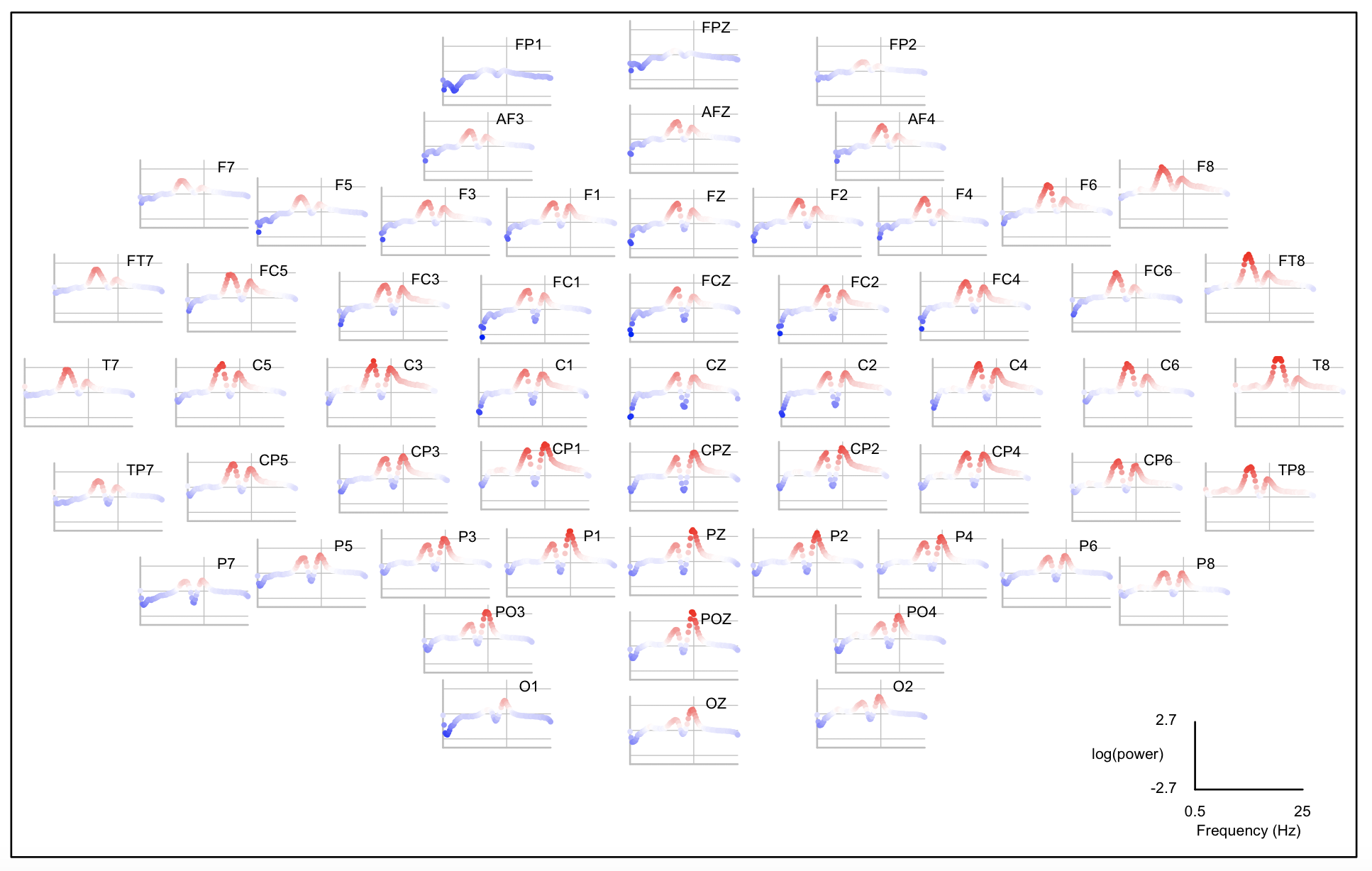
We'll use the lunaR ltopo.xy() routine to produce a plot of these data, first defining an additional variable as the signed -log10 of the empirical p-value:

d$S <- sign( d$B ) * -log10( d$PU )

The Luna graph command:

ltopo.xy( c=d$CH, x=d$F, y=d$S, z=d$S, pch=20, col=rbpal, cex=0.4, xline=15, yline=c(-2,0,2), y.symm=T)

then produces this plot where the Y-axis and also color-scaling show this scaled verson of the empirical significance:

Directly examining the PC column, we see there are 46 variables significant at 0.05 after correction:

table( d$PC < 0.05 )

and we can see which frequencies/channels they correspond to:

table( d$F[ d$PC < 0.05 ] , d$CH[ d$PC < 0.05 ] )

        C1 C2 CP1 CP2 CP3 CPZ CZ F1 F2 F4 FC1 FC2 FC3 FC4 FCZ Fp1 Fp2 FPZ FZ P2 POz PZ
  0.5    1  0   0   0   0   0  1  0  0  0   1   0   0   0   1   0   0   0  0  0   0  0
  0.75   1  1   0   1   1   1  1  1  1  1   1   1   1   1   1   1   1   1  1  1   0  1
  1      1  1   0   0   0   1  1  0  0  0   1   1   0   0   1   1   1   0  0  1   0  1
  1.25   0  0   0   0   0   0  1  0  0  0   0   0   0   0   0   0   0   0  0  0   0  0
  3      0  0   0   0   0   0  0  0  0  0   0   0   0   0   0   1   0   0  0  0   0  0
  3.25   0  0   0   0   0   0  0  0  0  0   0   0   0   0   0   1   0   0  0  0   0  0
  3.5    0  0   0   0   0   0  0  0  0  0   0   0   0   0   0   1   0   0  0  0   0  0
  15     0  0   0   0   0   0  0  0  0  0   0   0   0   0   0   0   0   0  0  0   1  0
  15.25  0  0   0   0   0   0  0  0  0  0   0   0   0   0   0   0   0   0  0  0   1  0
  15.5   0  0   1   0   0   0  0  0  0  0   0   0   0   0   0   0   0   0  0  0   1  0
  15.75  0  0   1   0   0   0  0  0  0  0   0   0   0   0   0   0   0   0  0  0   0  0
  16     0  0   1   0   0   0  0  0  0  0   0   0   0   0   0   0   0   0  0  0   0  0
  16.25  0  0   1   0   0   0  0  0  0  0   0   0   0   0   0   0   0   0  0  0   0  0

The console log notes there are two clusters significant at the empirical 0.05 level (after correction for all multiple testing, i.e. based on comparing the maximum of the cluster sum-statistics in the observed versus the permuted data). The p-values and seed variables can be obtained as follows:

destrat out.db +CPT -r K

ID   K   N    P         SEED
.    1   30   0.04495   CP4~16~PSD
.    2   33   0.01498   POz~15.25~PSD

(which note, does not include a cluster around 1 or 3 Hz). The members of each cluster can be found as follows:

destrat out.db +CPT -r K M

ID  K   M    VAR
.   1   1    C4~15.5~PSD
.   1   2    C4~15.75~PSD
.   1   3    C4~16.25~PSD
.   1   4    C4~16.5~PSD
.   1   5    C4~16~PSD
.   1   6    CP2~15.5~PSD
.   1   7    CP2~15.75~PSD
.   1   8    CP2~16.25~PSD
.   1   9    CP2~16.5~PSD
.   1   10   CP2~16~PSD
...

(or alternativelty, from the CLST variable in the point-wise output (-r VAR).

Warning

Further guidance on best practice on cluster thresholds, and implementing alternative methods to more intelligently select adaptive thresholds will be implemented in future releases. As is, please consider the clustering of the CPT as a secondary feature that has not been optimized in Luna yet: the primary application is to efficiently generate point-wise, corrected empirical p-values.