Time-series clustering

EXE

Epoch-by-epoch or channel-by-channel time-series clustering

This command provides an implementation of permutation distribution clustering, following Andreas Brandmaier's pdc R package. Within an individual, the EXE command can be applied to signal data, either within or between channels and/or epochs, to create a distance matrix that may likely be the starting point for subsequent clustering or dimension reduction approaches.

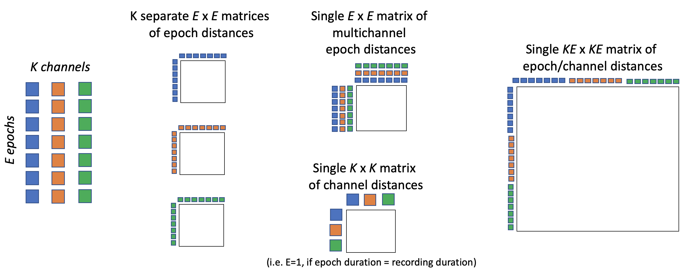
This command runs in one of four basic modes: for K channels and E epochs:

• univariate : K different channel-specific (ExE) matrics [uni]
• default : one combined multi-channel (ExE) matrix, i.e. a single distance metric for each pair of epochs is calculated based on the multivariate profiles of the K channels
• channel-wise : one channel-by-channel (KxK) matrix [cat with unepoched data ]
• concantenated : one matrix concatenating epochs from different channels (KExKE) [cat with epoched data, i.e running EPOCH beforehand ]

After forming one of these distance matrices, it can be output to a file for subsequent processing outside of Luna. Additionally, the EXE command can run hierarchical complete linkage clustering on this distance matrix.

Parameters

Other than specifying the type of distance matrix to be constructed (via cat, unit and the presence of a prior EPOCH command), you can change the default embedding dimension (m) and whether to skip samples (t).

Parameter	Example	Description
sig	sig=C3,C4	Specify channels
uni		Univariate (channel-by-channel) clstering of epochs
cat		Concatenate channels
mat	mat=f1	Dump distance matrix in file f1-{id}.mat
sr	sr=100	Change sample rate of signals prior to analysis
m	m=5	Permutation embedding dimension (valid values: 2 to 7)
t	t=1	Time delay between samples (default 1, no delay)

Hierarchical cluster analysis parameters:

Parameter	Example	Description
k	k=10	Maximum number of clusters (stopping rule)
mx	mx=20	Maximum cluster size

Extracting representative epochs heuristic:

Parameter	Example	Description
representative	representative=5	Select 5 representative epochs

Output

The primary output of EXE is the .mat text file, which is a tab-delimited distance matrix, containing the symmetric alpha-divergence distance measure (which is proportional to the squared Hellinger distance). For multi-channel data (K > 1), the distance is defined as the square root of the sum of squared single-channel distances.

In some conditions (with the cat option), there will be a corresponding .idx file, which describes the columns and rows of the distance matrix (in terms of which channels/epochs each reflects): i.e. containing an ID column and then CH (and optionally E also, if the data are epoched).)

If clustering was performed, the solution will be written to the default output mechanism:

Epoch-level cluster assignments (strata: E)

Variable	Description
CL	Cluster seed (epoch number)

If selecting representative epochs was performed, the additional outputs will be generated:

Epoch-level examplar assignments (strata: E)

Variable	Description
K	Exemplar/cluster number
KE	Epoch number of the exemplar

Class-level details (strata: K)

Variable	Description
E	Epoch number of this exemplar
N	Number of epochs associated w/ this exemplar

See below for an example of using the representative option.

Example

Here we estimate the epoch-by-epoch distance matrix for a single EEG channel in one individual:

luna s.lst 1 -o out.db -s 'EPOCH & EXE sig=C3 mat=d1 k=12'

If the individual's ID is id001, this will generate a file d1-id001.mat. We can then load this distance matrix into R, e.g.:

m <- as.matrix( read.table( "d1-id001.mat" ) ) 

We can also load the clusters that Luna assigned from the K = 12 hierarchical (complete linkage) clustering:

k <- ldb("out.db")
c <- k$EXE$E

The cluster each epoch is assigned to is in c$CL.

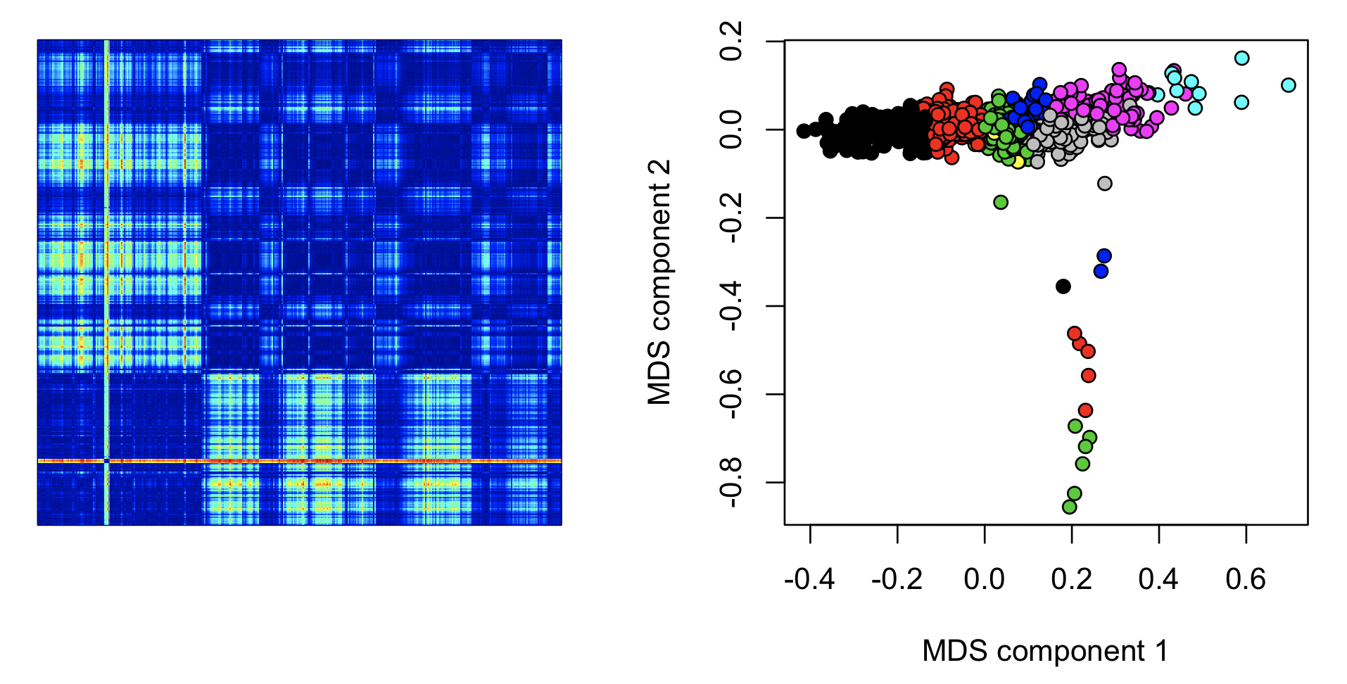
Here we plot the epoch-by-epoch distance matrix as a heat map (left), with the diagonal going from bottom left to top right. Second, we apply dimension reduction techniques such as multi-dimensional scaling, to produce metrics that might flag aberrent epochs (note: we just use a quick-and-dirty way to assign colors to clusters here, and sometimes different clusters are assigned the same color):

image(as.matrix(m), col = jet.colors(100) )
plot( cmdscale(as.dist(m)), xlab="MDS component 1", ylab="MDS component 2", pch=21, bg=as.factor( c$CL ) ) 

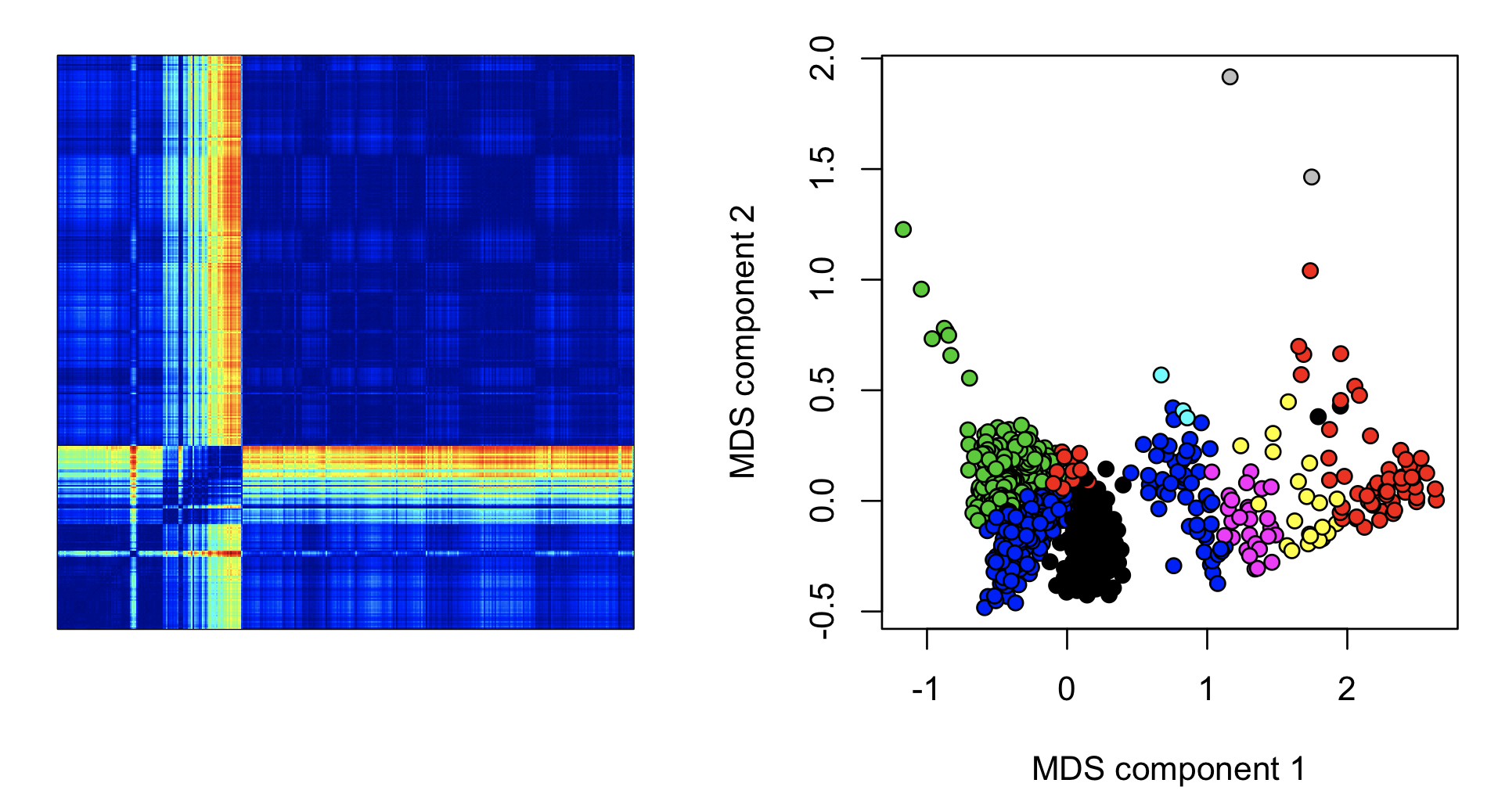
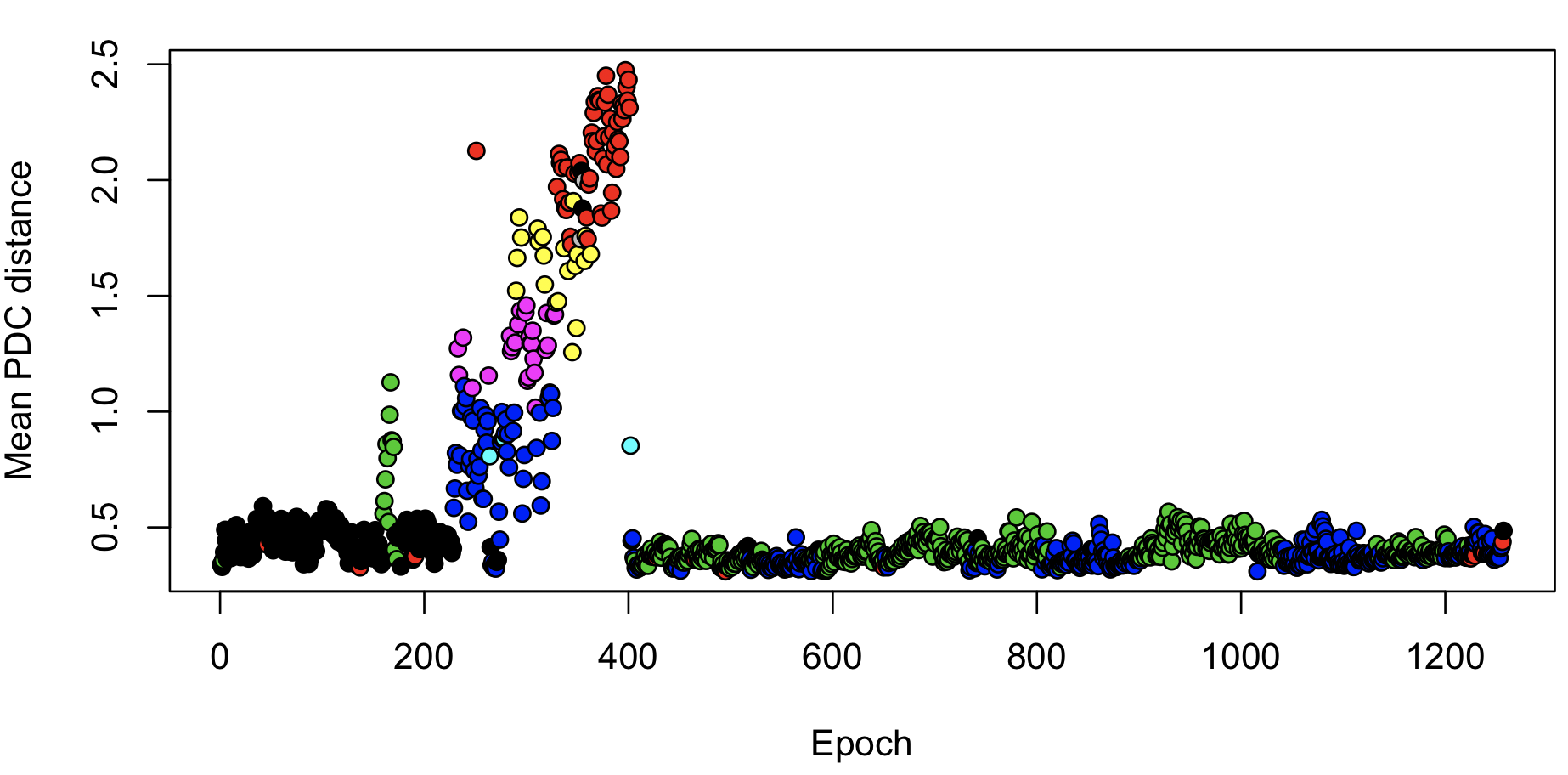
These types of epoch-wise (or channel-wise) analyses can potentially be useful in spotting (time-limited) aberrations in the data. Clearly there are some relatively unusual epochs starting about one third into the recording: the hotter colours (yellow/red) indicate that these epochs are more different compared to other epochs outside this interval, versus a random pair of epochs. Plotting the mean distance per epoch shows this effect around epochs 200 to 300: (nb. the banded assignment of epochs to the green, black or blue clusters from epoch 400 onwards presumably reflects differences in sleep stages.)

plot( apply(m, 1, mean), xlab="Epoch", ylab="Mean PDC distance", pch=21, bg=as.factor(c$CL) ) 

To get some more insight into this issue, we can look at raw data. First, we will look at the assignment of epochs to clusters:

table( c$CL ) 

 57 116 166 242 264 306 337 353 354 377 727 856 
226  16   8  53   3  27  21   2   2  58 529 312 

The top numbers (the values of c$CL, e.g. 57, etc) are the 'seeds' of each cluster, i.e. representing one epoch that was assigned to the cluster.

To look at the raw data for a given epoch, via lunaR, we can use ldata(). First, we randomly pick some epochs assigned to the cluster centered around epoch 242:

epochs <- sample( c$E[ c$CL == 242 ] , 5 )

Plotting 2 seconds worth of data from the first of these epochs (sample rate is 128 Hz):

plot( ldata( e=epochs[1] , chs="C3" )$C3[1:256]  , type = "l" )

Repeating this for typical epochs, we can view different examples of signals: e.g. here three instances from the unusual epochs (left / red) and three random ones from the rest of the sample (each for 2 seconds):

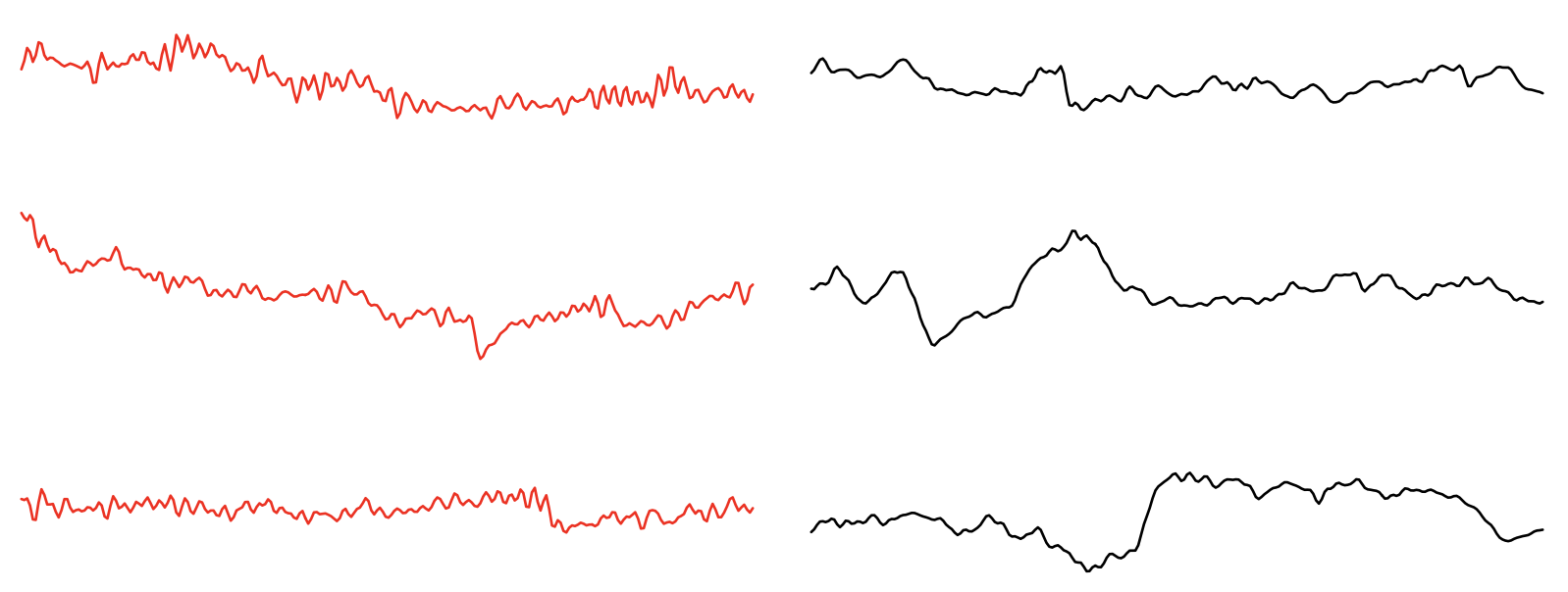
These examples point to some high-frequency interference during epochs ~200-300, not present in the rest of the signal (i.e. which made these epochs more similar). We can use lunaR to view the spectrogram for the C3 channel, up to 64 Hz:

lattach( lsl( "s.lst" )  , 1 )
k <- leval( "PSD sig=C3 epoch-spectrum max=64 dB" ) 
d <- k$PSD$CH_E_F 
lheatmap( d$E , d$F , d$PSD , col = jet.colors(100) ) 

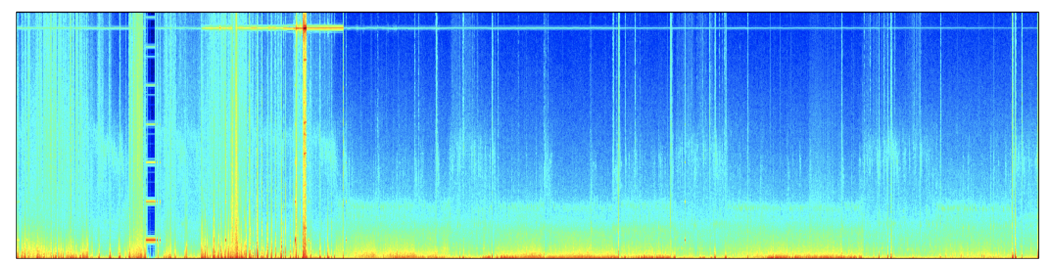
This points to a a constant electrical line noise artifact (the horizontal streak across the top of the spectrogram) which is amplified during the window from epoch 200 to 300. As a proof-of-principle, if we first band-pass filtered the signal prior to clustering:

luna s.lst 1 -o out.db -s 'EPOCH & FILTER sig=C3 bandpass=0.3,35 tw=0.5 ripple=0.02 & EXE sig=C3 mat=d1 k=12'

Now, we see a different structure in the data: the accentuated line-noise effect from epochs 200-300 has been removed; making two other feature of the data more visible: 1) a single small period of unusual epochs (that are also evident in the spectrogram), and 2) a long-range banding of similarity, which maps onto different stages of sleep (e.g. N3 epochs are more similar to other N3 epochs than to REM epochs, etc).

Note

We provide these examples simply to illustrate working with signal data and the EXE command, i.e. by itself, epoch-level time series clustering is probably not the most obvious way to QC sleep signal data.

Potential applications

The EXE command by itself is not particularly useful, but it can form the basis of other ways of looking at the data, i.e. any subsequent analysis that takes a distance matrix as its starting point, either between channels, epochs, and both.

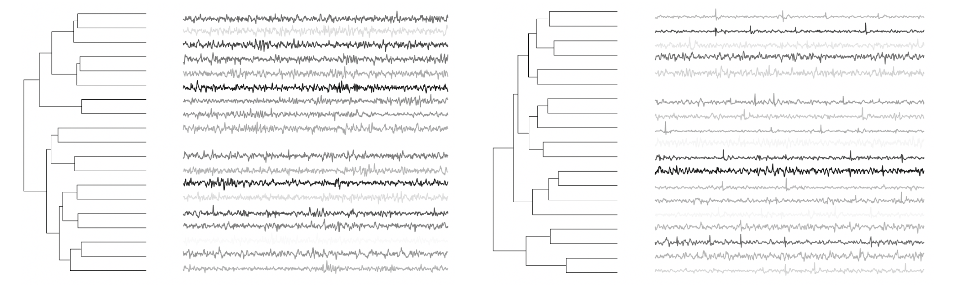
For example, here is one application in which hierarchical clustering (in sleep EEG from mice, with 10 second epochs) followed by affinity propagation clustering was used to generate exemplar epochs for each cluster (with the darkness of the trace being proportional to the frequency of the cluster). This provided a reasonably quick way to visually summarize more than 12 hours of data for each individual, for example showing one with basically clean data (left) versus one with a lot of recurrent artifact (right dendrogram).

A second class of application is to sanity check channels from polysomnography (PSG) studies. Different types of channels (EEG, EMG, ECG, respiratory, etc) will typically have somewhat distinctive signatures in terms of the permutation distributions (here using a fixed sample rate across different channels (via the RESAMPLE command) to allow distances across different types of channels:

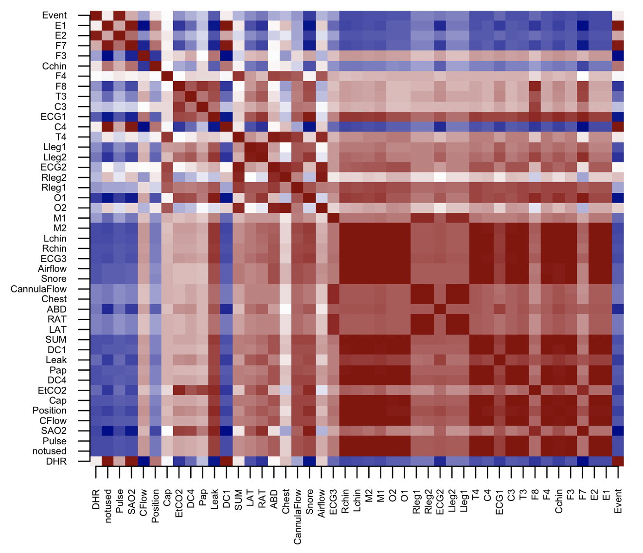
Plotting the dendrogram associated with this distance matrix, we see the tendency for like channels to cluster. If one or some channels have very high levels of artifact, they will cluster separately.

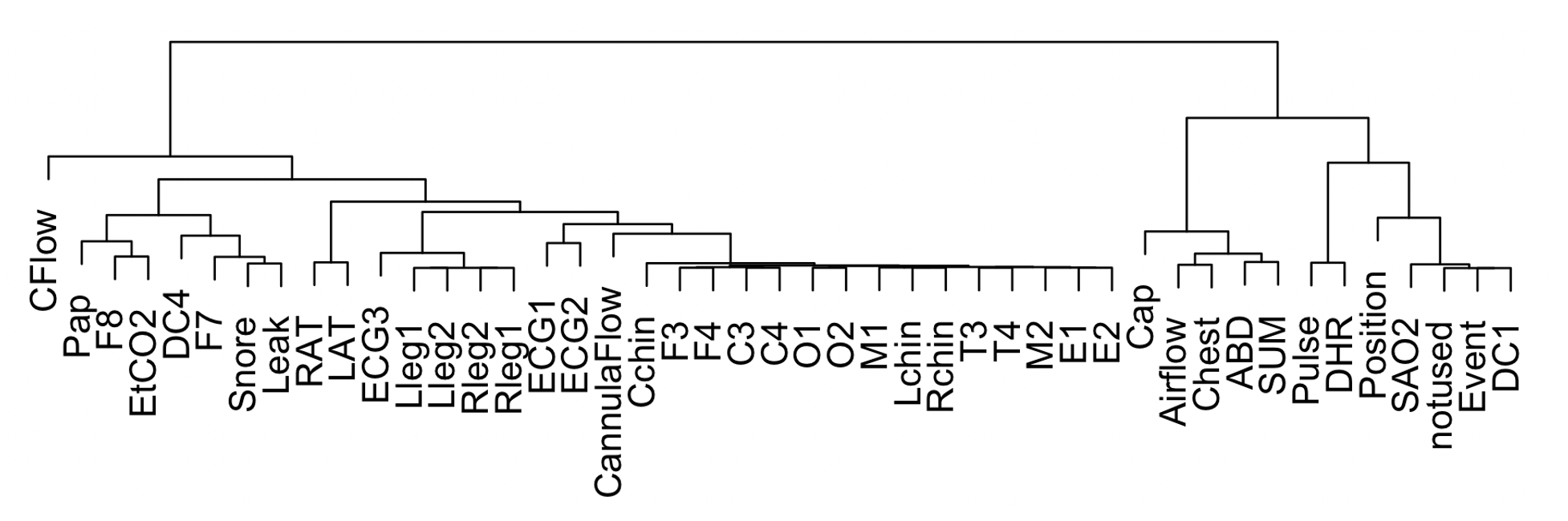
Although simply looking at the raw data would likely provide a quick and simple way to similarly spot gross artifact, these types of visual summaries may be useful in the context of automated pipelines that deal with large numbers of studies.

Representative epochs

The representative option (with argument k) will find k representative/exemplar epochs (and associate every epoch to the best-matching exemplar). This is conceptually similar to the hierarchical clustering approach. It uses a heuristic as described below.

The basic heuristic seeds on the epoch-by-epoch distance matrix, and iteratively makes splits of the epochs (using Otsu's method on the distribution of distances). For each split a representative epoch is selected as that which is most similar (lowest median distance) to all other epochs in that split. After making k splits, each epoch is assigned to the nearest representative/exemplar value.

luna s.lst -o out.db -s ' EPOCH & EXE sig=C3 representative=5 '

Note, it is necessary to explicitly EPOCH the data before running EXE representative.

Here, we see five splits, as requested, with exemplar epochs 1169, 294, etc.

destrat out.db +EXE -r K

ID      K    E      N
id01  1    1169   127
id01  2    294    396
id01  3    1305   199
id01  4    40     301
id01  5    318    341

destrat out.db +EXE -r E | head -15 

ID      E     K    KE
id01    1     4    40
id01    2     4    40
id01    3     4    40
id01    4     4    40
id01    5     4    40
id01    6     4    40
id01    7     4    40
id01    8     4    40
id01    9     5    318
id01    10    4    40
id01    11    4    40
id01    12    4    40
id01    13    4    40
id01    14    4    40
...

i.e. most of the initial epochs are assigned to class 4 (which has exemplar epoch 40). The exemplar epochs can be plotted to show a typical example of that class.

The Moonlight vewier has an EXE panel that implements EXE representative and shows the outputs: here it runs representative=5 to select five examplars. These are shown in the plots below (on the right - color-coded black, red, green, blue and cyan). The raw signal plotted above each is the 30-seconds signal of the exemplar epoch in each case. (The left plot is a heatmap of the distance matrix - with colder colors for less similar epochs):

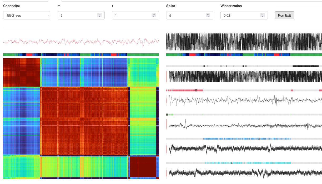
That is, the above output is based solely on running EXE representative as above.