POPS

Prediction of sleep stages

This page describes Luna's automated sleep stager (POPS). This vignette also gives some details on POPS and its companion command, SOAP. POPS is generic in the sense that it can be trained on multiple different types of signals.

The interactive Moonlight viewer provides a simple point-and-click interface to POPS (in prediction mode only), which is appropriate for applying our pre-made single-EEG POPS model to small numbers of EDFs. If using command-line Luna, the easiest place to start is with the RUN-POPS command.

Command	Description
Models	An overview of the current POPS models and expected signals
`RUN-POPS`	A high-level convenience wrapper around `POPS`
Moonlight	Instantiation of POPS base model in web-application
`POPS` prediction mode	Apply automated sleep stage prediction
`EVAL-STAGES`	Apply POPS evaluation metrics to external predictions
`--eval-stages`	Similar to above, but without an attached EDF
`POPS train` training mode (1)	Create level 1 feature matrices for training
`--pops` training mode (2)	Combine trainers for level 2 features and train POPS models

Models

An initial single EEG POPS model (s2) is hosted here:

URL = http://zzz.bwh.harvard.edu/dist/luna/pops.zip

Currently, we only distribute a single-EEG model however, although more will be added in the near future.

Download this ZIP file, and extract it to give a pops/ folder.

The model was trained on ~3500 individuals from the NSRR; although the model is a single-EEG model, both C3-M2 and C4-M1 channels were used, i.e. with the assumption that they are effectively interchangeable in this context. The models were trained using the workflow as described below. The next sections using either RUN-POPS or the lower-level POPS interface shows how to use these models for prediction.

The core s2 (aka Moonlight's M1, see below) model requires the following:

a single central EEG, based on a contralateral mastoid reference, i.e. C3-M2 or C4-M1. In practice, similar EEGs channels can be swapped in and should still perform similarly, e.g. F3-M2
channels must be band-pass filtered 0.3 - 35 Hz and sampled at 128 Hz
as well as this primary channel (which is given the placehold label CEN below), the s2 model expects a parallel, standardized version (called ZEN below), which can be obtained via the ROBUST-NORM Luna command

The s2 model can be used in two different ways (which correspond to the M1 and M2 labels in the Moonlight instantiation of POPS - both are based on the same underyling s2 model, however).

The default use takes a single EEG channel from the test subject and makes predictions
Alternatively, one can pass multiple comparable EEG channels to the prediction modules (e.g. C3-M2 and C4-M1); this uses the equiv POPS option to take both EEG channels, predict from each separately, and automatically select (epoch-by-epoch) the most "confident" prediction for each epoch

POPS files

When unzipping pops.zip (or creating new models from scratch), you'll see the following file types:

File	Description
`s2.ftr`	Feature file, specifying which features to compute per epoch from the raw EEG
`s2.mod`	Model file, generated by LightGBM after training the model
`s2.conf`	Configuration file, to control aspects of LightGBM when fitting the model
`s2.ranges`	Ranges file, represents the distribution of the training data
`s2.*.svd`	SVD files, specified by `s2.ftr` (used to project new data into the SVD component space )

Most users will only use POPS in prediction mode, which is simpler. Given a pre-trained model (as can be downloaded above) the core RUN-POPS command is in its most basic form just, e.g.:

RUN-POPS path=pops sig=C3_M2

See below for more details.

Training new models

However, if you want to train your own models (e.g. based on other populations, etc), you can use POPS in training mode without too much effort. The basic workflow for training POPS models is two-step:

  POPS train   
    - inputs: signals (EDFs) plus a feature definition file (.ftr)
    - output: epoch by (level 1) feature matrices (binary files)

  --pops
    - inputs: concatenated binary feature matrices & LGBM config (.conf) file
    - output: a `.mod` file (LGBM model) plus several auxiliaries, as above

The basic workflow for prediction using a previously created POPS model is a single step:

   POPS (or RUN-POPS)
    - inputs: signals (EDFs), feature, model files (.ftr,  .mod) & auxiliaries 
    - output: posterior probabilties & most likely stages per epoch

That is, the feature file (here s2.ftr) is a text file with a special syntax to specify which epoch-level features to extract from the raw signals. We use this s2.ftr feature file to both train models, and then also to predict in new individuals. That is, the feature files are the key link between the raw signal data, and the epoch-level feature matrix that is the fundamental data used in sleep staging by Luna. It is used both in training and in prediction. See below for a detailed overview. The .mod file is generated by LightGBM (the engine used to power POPS) and need not be inspected manually. The .conf file is not necessary when using RUN-POPS/POPS to predict sleep stages; otherwise, if the above files reside in the folder pops/ then

RUN-POPS

Wrapper around POPS for prediction

If using the standard POPS for prediction, it is necesary to perform a few steps to align signals with the channels that the s2 model is expecting, to mirror what was done during training:

create copies of the signals
to filter channels to the correct sample rate (128 Hz EEGs by default) (called CEN)
normalize a second copy of the signal using ROBUST-NORM (called ZEN)
to use the POPS model to make predictions

The RUN-POPS wrapper (the preferred way to use POPS) simplifies this, such that staging (for the s2 model) requires only a) one or more EEG signals and b) the location of the downloaded POPS models to be specified (e.g. assuming the base s2 model exists in the folder pops/):

luna s.lst -s ' RUN-POPS path=pops sig=C3_M2 '

In contrast, if using the lower-level POPS command, one might need to run something like this:

luna s.lst -s ' FILTER sig=C3_M2 bandpass=0.3,35 tw=0.5 ripple=0.02
                COPY sig=C3_M2 tag=NORM
                ROBUST-NORM sig=C3_M2_NORM epoch winsor=0.005 second-norm=T
                POPS alias=CEN,ZEN|C3_M2,C3_M2_NORM path=pops lib=s2 '

and this would become more involved if apply multiple equivalance channels.

Parameters

Epoch-level confusion matrix (strata: OBS x PRED)

Parameter	Example	Description
`path`	`/home/user/data/pops/`	Path to POPS model folder (downloaded)
`lib`	`m2`	Optionall, a POPS model (default `s2`)
`sig`	`C3`	One or more EEG signals
`ref`	`M2`	Optionally, one of more references (matching `sig`)
`args`	`args="op1=val1 op2=val2"`	Pass other arguments to POPS
`ignore-obs`	`T`	Ignore any observed staging (default: `F`)
`filter`	`F`	Filter signals 0.3 - 35 Hz (default: `T` )
`edger`	`F`	Whether to perform EDGER trimming prior to prediction (default: `T`)

Outputs

See the POPS command outputs below.

Example

If we need to reference the channel on-the-fly:

luna s.lst -s ' RUN-POPS path=pops sig=C3 ref=M2 '

For multiple equivalence channels:

luna s.lst -s ' RUN-POPS path=pops sig=C3_M2,C4_M1 '

For multiple equivalence channels and also perform re-referencing (the i-th entry in sig is referenced against the i-th entry in ref):

luna s.lst -s ' RUN-POPS path=pops sig=C3,C4 ref=M2,M1 '

For a specific example, applied to a tutorial dataset EDF:

luna s.lst 2 -o out.db -s RUN-POPS sig=EEG path=~/dropbox/pops

This shows the steps RUN-POPS performs in the log:

 CMD #1: RUN-POPS
   options: path=/Users/smp37/dropbox/pops sig=EEG
  ------------------------------------------------------------
  making copies of original signals (appending _F)
  copying EEG to EEG_F
  ------------------------------------------------------------
  resampling EEG_F to 128 Hz if needed
  resampling channel EEG_F from sample rate 125 to 128
  ------------------------------------------------------------
  bandpass filtering signals
  filtering channel(s): EEG_F
  ------------------------------------------------------------
  making time-domain normalized signals
  copying EEG_F to EEG_F_N
  set epochs to default 30 seconds, 1195 epochs
  iterating over epochs
  robust standardization of 1 signals, winsorizing at 0.002
  ------------------------------------------------------------
  scanning to trim excess leading/trailing wake/artifact
  skipping... cache ec1 not found for this individual...
  set 0 leading/trailing sleep epochs to '?' (given end-wake=120 and end-sleep=5)
  anchoring on sleep epochs only for normative ranges, using 715 of 1195 epochs
  for EEG_F, flagged 340 epochs (H1=270, H3=96)
  H(1) bounds: 3.58812 .. 6.97429
  H(3) bounds: 0.299615 .. 0.928851
  setting cache ec1 to store times
  lights-on=05.13.06 (skipping 244 epochs from end)
  ------------------------------------------------------------

It then applies the POPS command:

  running POPS
  reading feature specification from /Users/smp37/dropbox/pops/s2.ftr
   396 level-1 features, 109 level-2 features
   113 of 505 features selected in the final feature set
  read 65 valid feature mean/SD ranges from /Users/smp37/dropbox/pops/s2.ranges
  from TRIM cache, setting lights_on = 28500 secs, 475 mins from start
  set 245 final epochs to L based on a lights_on time of 28500 seconds from EDF start
  set 0 leading/trailing sleep epochs to '?' (given end-wake=120 and end-sleep=5)
  existing staging found: will calculate predicted/observed agreement metrics
  expecting 396 level-1 features (for 1195 epochs) and 2 signals
  applying Welch with 4s segments (2s overlap), using median over segments
  pruning rows from 1195 to 950 epochs
  feature matrix: 950 rows (epochs) and 113 columns (features)
  set 20 ( prop = 0.000186306) data points to missing
  read model from /Users/smp37/dropbox/pops/s2.mod (1000 iterations)
  adding POPS annotations (pN1, pN2, pN3, pR, pW, p?)

  kappa = 0.830578; 3-class kappa = 0.860016 (n = 950 epochs)

  Confusion matrix: 
       Pred:    W      R     N1     N2     N3     Tot
  Obs:   W    224      1      8      3      0    0.25
         R      1     99      4     16      0    0.13
        N1      4      0      5      2      0    0.01
        N2     14     18      8    329     29    0.42
        N3      2      0      0      6    177    0.19
      Tot:   0.26   0.12   0.03   0.37   0.22    1.00

The output database will now have the same output as described for POPS below, except the command name is RUN-POPS here and not POPS:

destrat out.db +RUN-POPS -v K K3

ID        K           K3
nsrr02    0.830578    0.860016

The epoch-level predictions are obtained as follows:

destrat out.db +RUN-POPS -r E -v PP_N1 PP_N2 PP_N3 PP_R PP_W PRED PRIOR

ID      E     PP_N1   PP_N2   PP_N3    PP_R    PP_W  PRED PRIOR
   ...
nsrr02  553   0.004   0.673   0.318   0.002   0.003    N2    N2
nsrr02  554   0.002   0.511   0.482   0.001   0.003    N2    N2
nsrr02  555   0.002   0.369   0.627   0.001   0.002    N3    N2
nsrr02  556   0.003   0.591   0.402   0.001   0.003    N2    N2
nsrr02  557   0.002   0.525   0.470   0.001   0.002    N2    N3
nsrr02  558   0.002   0.548   0.445   0.001   0.003    N2    N2
nsrr02  559   0.001   0.327   0.669   0.001   0.002    N3    N2
nsrr02  560   0.002   0.351   0.644   0.001   0.002    N3    N3
nsrr02  561   0.004   0.341   0.651   0.002   0.003    N3    N2
nsrr02  562   0.002   0.270   0.725   0.001   0.002    N3    N2
nsrr02  563   0.002   0.250   0.745   0.001   0.002    N3    N2
nsrr02  564   0.002   0.251   0.744   0.001   0.002    N3    N2
nsrr02  565   0.002   0.345   0.649   0.001   0.002    N3    N2
nsrr02  566   0.002   0.279   0.715   0.001   0.003    N3    N3
nsrr02  567   0.002   0.337   0.657   0.001   0.002    N3    N2
nsrr02  568   0.001   0.194   0.802   0.001   0.002    N3    N2
nsrr02  569   0.001   0.164   0.833   0.001   0.002    N3    N3
nsrr02  570   0.003   0.300   0.693   0.002   0.003    N3    N2
nsrr02  571   0.001   0.282   0.713   0.001   0.002    N3    N3
nsrr02  572   0.002   0.307   0.687   0.002   0.002    N3    N3
nsrr02  573   0.001   0.284   0.711   0.002   0.002    N3    N3
nsrr02  574   0.003   0.322   0.670   0.002   0.002    N3    N2
nsrr02  575   0.005   0.317   0.672   0.003   0.003    N3    N2
nsrr02  576   0.010   0.711   0.269   0.005   0.005    N2    N2
nsrr02  577   0.002   0.311   0.683   0.002   0.003    N3    N3
nsrr02  578   0.001   0.232   0.764   0.002   0.002    N3    N2
nsrr02  579   0.003   0.294   0.698   0.002   0.004    N3    N3
nsrr02  580   0.005   0.520   0.469   0.003   0.003    N2    N2
nsrr02  581   0.004   0.647   0.344   0.002   0.003    N2    N2
nsrr02  582   0.002   0.329   0.663   0.002   0.003    N3    N3
nsrr02  583   0.004   0.455   0.532   0.005   0.004    N3    N2
nsrr02  584   0.003   0.147   0.838   0.007   0.005    N3    N3
nsrr02  585   0.008   0.202   0.765   0.017   0.009    N3    N3
nsrr02  586   0.026   0.236   0.692   0.032   0.014    N3    N3
nsrr02  587   0.021   0.037   0.005   0.009   0.926     W     W
nsrr02  588   0.021   0.017   0.002   0.005   0.955     W     W
...

POPS (prediction)

Single observation stage accuracies and probabilities

Note that the RUN-POPS wrapper provides a simpler way to call the POPS stager in prediction mode, and should generally be the preferred route.

Parameters

Primary options:

Option	Example	Description
`path`	`/path/to/pops`	Folder where POPS feature, model files, etc reside
`lib`	`s2`	Name of library in `path` folder (i.e. root for `.ftr`, `.mod`, etc
`alias`	`CEN,ZEN\|C3_M2,C3_M2_NORM`	Assign `CEN` (from `.ftr`) to be `C3_M2` (from EDF), etc
`equiv`	`CEN,ZEN\|C4_M1,C4_M1_NORM`	Use `C4_M1` as a second equivalent alongside the original `CEN`; likewise for `C4_M1_NORM` and `ZEN`
`replace`	`CEN,C3`	Replace EDF channel `CEN` with `C3`
`lights-off`	`23:00:00`	Lights off time (ignore epochs before)
`lights-on`	`08:00:00`	Lights on time (ignore epochs after)
`SHAP`		Estimate SHAP information scores (takes longer to run)
`SHAP-epoch`		Estimate epoch-level SHAP information scores (takes longer to run & verbose output)

Output

The primary output of running POPS in prediction mode is a set of posterior probabilities for each epoch, along with the most likely stage.

If the dataset contained manual staging, Luna will also report a suite of accuracy measures and print confusion matrices to the console (i.e. on the assumption that the original staging represent a gold standard).

In addition, POPS adds a set of annotations - labelled either N1, N2, N3, R and W (if no original staging present), or pN1, pN2, pN3,pR and pW if there was original staging. In practice, one may there want to add a command such as

WRITE-ANNOTS annot=pN1,pN2,pN3,pR,pW file=^-pops.annot hms '

after running POPS to make predictions. If output with p (POPS) prefixes, you can tell Luna to use those as the standard staging annotations via ss-prefix=p (or ss-pops=T: i.e. this will use POPS staging if the file pops.annot was previously generated in id1-pops.annot:

luna s.lst ss-prefix=p annot-file=id1-pops.annot -s HYPNO

Individual-level output (strata: none)

Variable	Description
`ACC`	Accuracy
`ACC3`	3-class accuracy (NR/R/W)
`K`	Kappa
`K3`	3-class Kappa
`MCC`	Matthew's correlation coef.
`MCC3`	3-class MCC
`F1`	F-1 score
`F13`	3-class F-1 score
`F_WGT`	Weighted F-1
`RECALL`	Recall
`RECALL3`	3-class recall
`RECALL_WGT`	Weighted recall
`PREC`	Precision
`PREC3`	3-class precision
`PREC_WGT`	Weighted precision
`REM_LAT_OBS`	Observed REM latency
`REM_LAT_PRD`	Predicted REM latency
`SLP_LAT_OBS`	Observed sleep latency
`SLP_LAT_PRD`	Predicted sleep latency

Epoch-level outputs (stratum: E)

Variable	Description
`PRIOR`	Prior staging, if present
`PRED`	Predicted (most likely) stage
`CONF`	Confidence score (highest posterior)
`FLAG`	Flagged if an issue/outlier (0/1)
`START`	Start time of epoch
`STOP`	Start time of epoch
`PP_N1`	Posterior probability, N1
`PP_N2`	Posterior probability, N2
`PP_N3`	Posterior probability, N3
`PP_R`	Posterior probability, REM
`PP_W`	Posterior probability, wake

Stage-specific metrics (stratum: SS )

Variable	Description
`ORIG`	Stage duration, original staging
`PRF`	Stage duration, predicted, weighted by posteriors
`PR1`	Stage duration, predicted, counting most-likely epochs
`F1`	F-1 score
`PREC`	Precision
`RECALL`	Recall
`OBS`	Number of observations

Feature-level summaries (stratum: FTR)

Variable	Description
`LABEL`	Feature label
`LABEL_ORIG`	Original label
`INC`	Included? 0/1
`DROPPED`	Dropped? 0/1
`FINAL`	Column number in final feature matrix, if present
`LEVEL`	Level 1 or level 2 feature?
`BAD`	Bad feature (outliers)?
`BLOCK`	Block label
`PROP`	Proportion of missing observations
`ROOT`	Label root name

Epoch-level accuracy by transition class (stratum: ETYPE)

Variable	Description
`ACC`	Accuracy
`N`	Number of events

See the SOAP documentation for a description of the various ETYPE levels.

Stage-specific epoch-level accuracy by transition class (strata: SS x ETYPE)

Variable	Description
`ACC`	Accuracy
`N`	Number of events

SHAP information scores (strata: SS x FTR)x

Variable	Description
`SHAP`	SHAP value for that stage/feature

Epoch-level confusion matrix (strata: OBS x PRED)

Variable	Description
`N`	Number of epochs
`P_COND_OBS`	Probability of predicted stage, conditional on observed stage
`P_COND_PRED`	Probability of observed stage, conditional on predicted stage

Example

Taking the second individual from the tutorial dataset:

luna s.lst 2 -o out.db \
            -s ' FILTER sig=EEG bandpass=0.3,35 tw=0.5 ripple=0.02
                 COPY sig=EEG tag=NORM
                 ROBUST-NORM sig=EEG_NORM epoch winsor=0.005 second-norm=T
                 POPS alias=CEN,ZEN|EEG,EEG_NORM path=pops lib=s2
                 WRITE-ANNOTS annot=pN1,pN2,pN3,pR,pW file=pops.annot hms '

This gives some verbose information to the console, describing the creation of the feature matrix:

  reading feature specification from pops/s2.ftr
   396 level-1 features, 109 level-2 features
   113 of 505 features selected in the final feature set
  read 65 valid feature mean/SD ranges from pops/s2.ranges
  set 0 leading/trailing sleep epochs to '?' (given end-wake=120 and end-sleep=5)
  expecting 396 level-1 features (for 1195 epochs) and 2 signals
  applying Welch with 4s segments (2s overlap), using median over segments
  resampling channel EEG from sample rate 125 to 128
  resampling channel EEG_NORM from sample rate 125 to 128
  pruning rows from 1195 to 1195 epochs
   - adding level-2 feature SVD: SPEC1 (n=98) --> SPEC1.SVD (n=6, cols:396-401) 
   - reading SVD W and V from pops/s2.spec1.svd
   - adding level-2 feature SVD: SPEC2 (n=98) --> SPEC2.SVD (n=6, cols:402-407) 
   - reading SVD W and V from pops/s2.spec2.svd
   - adding level-2 feature SVD: RSPEC1 (n=98) --> RSPEC1.SVD (n=4, cols:408-411) 
   - reading SVD W and V from pops/s2.rspec1.svd
   - adding level-2 feature SVD: RSPEC2 (n=98) --> RSPEC2.SVD (n=4, cols:412-415) 
   - reading SVD W and V from pops/s2.rspec2.svd
   - adding level-2 feature SMOOTH: SPEC1.SVD (n=6) --> SPEC1.SVD.SMOOTHED1 (n=6, cols:416-421) 
   - adding level-2 feature SMOOTH: SPEC2.SVD (n=6) --> SPEC2.SVD.SMOOTHED1 (n=6, cols:422-427) 
   - adding level-2 feature SMOOTH: MISC1 (n=4) --> MISC1.SMOOTHED1 (n=4, cols:428-431) 
   - adding level-2 feature SMOOTH: SPEC1.SVD (n=6) --> SPEC1.SVD.SMOOTHED2 (n=6, cols:432-437) 
   - adding level-2 feature SMOOTH: SPEC2.SVD (n=6) --> SPEC2.SVD.SMOOTHED2 (n=6, cols:438-443) 
   - adding level-2 feature SMOOTH: MISC1 (n=4) --> MISC1.SMOOTHED2 (n=4, cols:444-447) 
   - adding level-2 feature SMOOTH: SPEC1.SVD (n=6) --> SPEC1.SVD.SMOOTHED3 (n=6, cols:448-453) 
   - adding level-2 feature SMOOTH: SPEC2.SVD (n=6) --> SPEC2.SVD.SMOOTHED3 (n=6, cols:454-459) 
   - adding level-2 feature SMOOTH: MISC1 (n=4) --> MISC1.SMOOTHED3 (n=4, cols:460-463) 
   - adding level-2 feature SMOOTH: RSPEC1.SVD (n=4) --> RSPEC1.SVD.SMOOTHED1 (n=4, cols:464-467) 
   - adding level-2 feature SMOOTH: RSPEC2.SVD (n=4) --> RSPEC2.SVD.SMOOTHED1 (n=4, cols:468-471) 
   - adding level-2 feature SMOOTH: RSPEC1.SVD (n=4) --> RSPEC1.SVD.SMOOTHED2 (n=4, cols:472-475) 
   - adding level-2 feature SMOOTH: RSPEC2.SVD (n=4) --> RSPEC2.SVD.SMOOTHED2 (n=4, cols:476-479) 
   - adding level-2 feature SMOOTH: RSPEC1.SVD (n=4) --> RSPEC1.SVD.SMOOTHED3 (n=4, cols:480-483) 
   - adding level-2 feature SMOOTH: RSPEC2.SVD (n=4) --> RSPEC2.SVD.SMOOTHED3 (n=4, cols:484-487) 
   - adding level-2 feature NORM: MISC1 (n=4) --> ZMISC1 (n=4, cols:488-491) 
   - adding level-2 feature NORM: MISC1.SMOOTHED1 (n=4) --> ZMISC1.SMOOTHED1 (n=4, cols:492-495) 
   - adding level-2 feature NORM: MISC1.SMOOTHED2 (n=4) --> ZMISC1.SMOOTHED2 (n=4, cols:496-499) 
   - adding level-2 feature NORM: MISC1.SMOOTHED3 (n=4) --> ZMISC1.SMOOTHED3 (n=4, cols:500-503) 
   - adding level-2 feature TIME: --> TIME1 (n=1, cols:504-504) 
  feature matrix: 1195 rows (epochs) and 113 columns (features)
  set 1765 ( prop = 0.0130707) data points to missing
  read model from pops/s2.mod (1000 iterations)

After making the predictions, POPS create the annotations, and outputs the kappa (if there are observed staging data);

  adding POPS annotations (pN1, pN2, pN3, pR, pW)
  kappa = 0.821632; 3-class kappa = 0.871336 (n = 1195 epochs)

Note that these are the same kappas are output by Moonlight above.

This also prints the 5-class confusion matrix:

  Confusion matrix: 
       Pred:      W      R    N1      N2     N3    Tot
  Obs:  W       465      1    13       1      0    0.4
        R         0    117     2       1      0    0.1
       N1         5      1     4       1      0   0.01
       N2        14     53    11     312      9   0.33
       N3         1      0     0      37    147   0.15
     Tot:      0.41   0.14   0.03   0.29   0.13    1.0

  Confusion matrix: 
    Pred:      W      R     N1     N2     N3    Tot
  Obs:   W   465      1     13      1      0    0.4  
         R     0    117      2      1      0    0.1 
        N1     5      1      4      1      0   0.01
        N2    14     53     11    312      9   0.33
        N3     1      0      0     37    147   0.15
       Tot: 0.41   0.14   0.03   0.29   0.13    1.0

In this instance, the kappa is quite high (0.82 for 5-class, and 0.87 for the 3-class instance). Naturally, depending on a) the depth/consistency of sleep, b) the quality of the signals and c) any other technical differences between the test data and the training data, the performance might not be as good.

For example, applying the same model to the first tutorial individual, the initial kappa is much lower (<0.4). However, this is in large part because of an extend period of artifact after the lights-on period of the recording. Setting the lights-on option to exclude that increases the accuracy of prediction quite a lot. (This is because of the normalization step involved in pre-processing.) We'll be adding some vignettes in the future to consider best practice for applying POPS, adding new models (e.g. including EOGs, EMGs, etc).

Moonlight

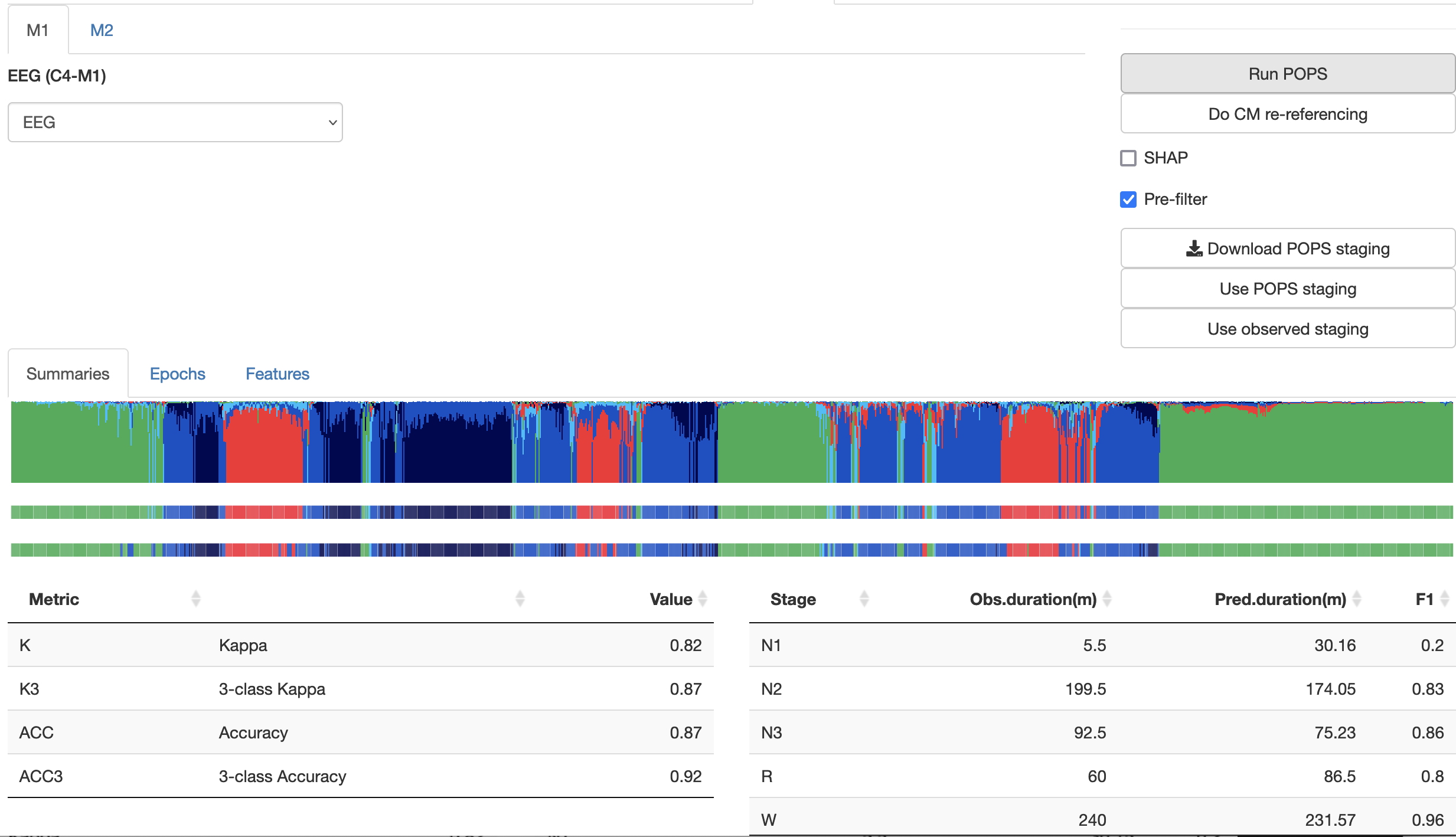
One easy route to use POPS (at least for small numbers of EDFs) is the point-and-click Moonlight tool. Opening the Hypnogram/POPS panel, we can select the M1 model (which actually maps to the s2 model described above), specify the single channel to use (EEG, which is C4-M1), and check that we need to bandpass the signal prior to staging). Click Run POPS and then 5-10 seconds later, you'll have this output;

The epoch-level predictions are available in a table from the second sub-panel too:

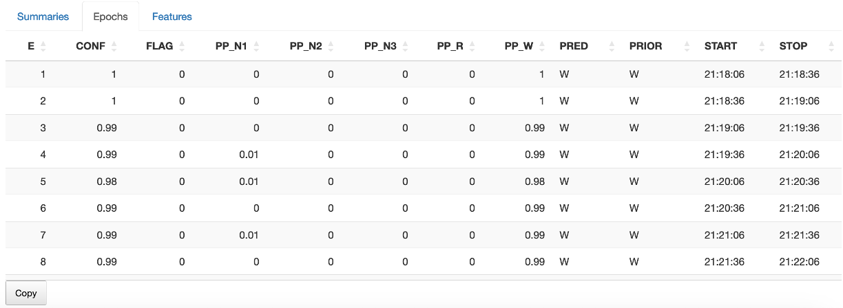
(It is also possible to set lights-off/on times (approximately anyway) by selecting and dragging the mouse on the top hypnogram - see the main Moonlight tutorial).

However, if you are wishing to a) use different models, b) alter parameters, and/or c) stage more than a handful of studies in a reproducible manner, then it is highly advised (and ultimately, much easier) to use the standard command line Luna tool, as described above.

EVAL-STAGES

Evaluates an external set of stages against the internal set

Given an external file (in .eannot format) of predicted stages, this command will read those, and compare them to the observed stages (i.e. from the original annotations) and generate the same table of statistics as POPS outputs.

Parameters

Option	Example	Description
`file`	`stage.txt`	File with staging

Output

The key outputs are also for POPS (kappas, accuracies and confusion matrices). See above.

Example

If we had extracted the annotations from the previous POPS predictions into the file stage.txt as an .eannot, the following command would give the same metrics as the original POPS command:

luna s.lst 2 -o out.db -s EVAL-STAGES file=stage.txt

  kappa = 0.821632; 3-class kappa = 0.871336 (n = 1195 epochs)
  Confusion matrix: 
    Pred:      W       R     N1     N2     N3    Tot
  Obs:   W   465       1     13      1      0    0.4
         R     0     117      2      1      0    0.1
        N1     5       1      4      1      0   0.01
        N2    14      53     11    312      9   0.33
        N3     1       0      0     37    147   0.15
      Tot:   0.41   0.14   0.03   0.29   0.13   1.00

i.e. EVAL-STAGES just performs the last comparison steps of POPS, but rather than using the POPS model to generate the predictions, it swaps in an external set of predictions. This can be useful, for example, if you want to compare the performance of another stager, on the same exact set of metrics as POPS.

--eval-stages

Evaluates an external set of stages against another external set

This is similar to EVAL-STAGES except there is no attached EDF/annotation set. It simply takes two .eannot style files of stages (one row per epoch) of the same length, and generates agreement statistics.

Parameters

Option	Example	Description
`file`	`stage.txt`	File with staging
`file2`	`stage2.txt`	Second file with staging

Output

As above.

Example

luna --eval-stages --opt file=stages1.txt file2=stages2.txt

POPS (training)

Flexibly specify and train new POPS models

This is an advanced section, that covers using POPS to generate one's own stager.

Feature files

Although understanding the details of POPS feature files is not necessary in order to use POPS to predict new stages, it is useful to review briefly.

Here are the features understood by POPS:

Level 1 features:

Features	Arguments	Description
`SPEC`		Power (default 0.25 Hz bins from 4-sec window)
`RSPEC`		Relative power
`VSPEC`		Intra-epoch variance in power
`BAND`		Band power
`RBAND`		Relative band power
`VBAND`		Intra-epoch variance in band power
`COH`		Magnitude-squared coherence
`SLOPE`		Spectral slope (30-45 Hz)
`SKEW`		Skewness
`KURTOSIS`		Kurstosis
`HJORTH`		Hjorth parameters
`FD`		Fractal dimension
`PE`	`from` `to`	Permutation entropy (order 3 to 7)
`MEAN`		Epoch mean
`OUTLIERS`	`th`	Remove outlier epochs
`COVAR`		Individual-level/demographic covariates (from `vars`)

Level 2 features:

Feature	Arguments	Description
`TIME`	`order`	Time track
`SMOOTH`	`block` `half-window` `a`	Smoothing window
`DENOISE`	`block` `lambda=0.5`	Total-variation denoiser
`SVD`	`block` `nc` `file`	PCA/SVD
`NORM`	`block`	Normalize
`RESCALE`	`block`
`CUMUL`	`block`	Make epoch-level cumulative features
`DERIV`	`block`	Make epoch-level derivative features

Here is the main s2.ftr file (with comments interleaved):

% --------------------------------------------------------------------------------
% Declare any channels used (required), sample rates
% --------------------------------------------------------------------------------

% trained channel label = generic 'CEN'
%  CEN central EEG, filtered
%  ZEN central EEG, normed

CH CEN 128 uV
CH ZEN 128 uV

It is possible to specify aliases for CEN and ZEN (i.e. these are effectively placeholder labels) in the .ftr file (e.g. CH CEN C3_M2 C4_M1 128 uV) but as above, we can also use the alias option for POPS to do this for a given dataset.

Next, we specify some main level 1 features: i.e. the core features calculated independently per individual:

% --------------------------------------------------------------------------------
% Level 1 features
%  block : feature {key=value key=value}
% --------------------------------------------------------------------------------

spec1: SPEC     CEN lwr=0.75 upr=25 
spec2: SPEC     ZEN lwr=0.75 upr=25 

rspec1: RSPEC    CEN lwr=0.75 upr=25 z-lwr=0.75 z-upr=25
rspec2: RSPEC    ZEN lwr=0.75 upr=25 z-lwr=0.75 z-upr=25

misc1: FD       ZEN 
misc1: PE       ZEN from=4 to=4
misc1: HJORTH   ZEN

The full table of features is given below. Note that the features are assigned to a block (e.g. spec1). This is an arbitrary label that can be used in the feature definition file to refer to the set of features. For example, spec1 maps to 98 columns from 0.75 Hz to 25 Hz in (by default) 0.25 Hz increments.

We next specify that epochs will be removed if any feature contains an extreme outlier value (10 SD units):

% --------------------------------------------------------------------------------
% Epoch/row exclusions based on level-1 features
% --------------------------------------------------------------------------------

misc1: OUTLIERS th=10

Level 2 features are based on level 1 features for one or more individuals. These are calculated on-the-fly when training models; they may also involve data reduction methods (SVD) that depend on multiple individuals, as below:

% --------------------------------------------------------------------------------
% Level 2 features: 
%  to-block: feature block=from-block {key=value}
% --------------------------------------------------------------------------------

spec1.svd:  SVD block=spec1  nc=6 file=s2.spec1.svd
spec2.svd:  SVD block=spec2  nc=6 file=s2.spec2.svd

rspec1.svd:  SVD block=rspec1  nc=4 file=s2.rspec1.svd
rspec2.svd:  SVD block=rspec2  nc=4 file=s2.rspec2.svd

That is, the SVD command takes all the variables in the spec1 block, normalizes within individual, fits a single SVD across all epochs/all individuals, and then extracts the top 6 components; in training mode, Luna will save the SVD to the file s2.spec1.svd; in prediction mode, Luna will read s2.spec1.svd and use it to project to derive the 6 new variables (i.e. summaries of the original 98 spectral values, in this case).

Next, we apply some temporal smoothing -

% --------------------------------------------------------------------------------
% Temporal smoothing
% --------------------------------------------------------------------------------

spec1.svd.smoothed1:  SMOOTH block=spec1.svd  half-window=2
spec2.svd.smoothed1:  SMOOTH block=spec2.svd  half-window=2
misc1.smoothed1:      SMOOTH block=misc1      half-window=2

spec1.svd.smoothed2:  SMOOTH block=spec1.svd  half-window=10
spec2.svd.smoothed2:  SMOOTH block=spec2.svd  half-window=10
misc1.smoothed2:      SMOOTH block=misc1      half-window=10

spec1.svd.smoothed3:  SMOOTH block=spec1.svd  half-window=25
spec2.svd.smoothed3:  SMOOTH block=spec2.svd  half-window=25
misc1.smoothed3:      SMOOTH block=misc1      half-window=25

rspec1.svd.smoothed1:  SMOOTH block=rspec1.svd  half-window=2
rspec2.svd.smoothed1:  SMOOTH block=rspec2.svd  half-window=2

rspec1.svd.smoothed2:  SMOOTH block=rspec1.svd  half-window=10
rspec2.svd.smoothed2:  SMOOTH block=rspec2.svd  half-window=10

rspec1.svd.smoothed3:  SMOOTH block=rspec1.svd  half-window=25
rspec2.svd.smoothed3:  SMOOTH block=rspec2.svd  half-window=25

We next normalize some of the smooth metrics:

% --------------------------------------------------------------------------------
% Normalize 
% --------------------------------------------------------------------------------

zmisc1:   NORM block=misc1
zmisc1.smoothed1:   NORM block=misc1.smoothed1
zmisc1.smoothed2:   NORM block=misc1.smoothed2
zmisc1.smoothed3:   NORM block=misc1.smoothed3

We add a time track (elapsed time from EDF start, scaled from -0.5 to +0.5):

% --------------------------------------------------------------------------------
% Time track
% --------------------------------------------------------------------------------

time1: TIME

Finally, we select the subset of blocks to be used in the final model:

% --------------------------------------------------------------------------------
%
% Final feature selection (blocks as defined above)
%
% --------------------------------------------------------------------------------

SELECT spec1.svd  spec1.svd.smoothed1 spec1.svd.smoothed2 spec1.svd.smoothed3
SELECT spec2.svd  spec2.svd.smoothed1 spec2.svd.smoothed2 spec2.svd.smoothed3

SELECT rspec1.svd  rspec1.svd.smoothed1 rspec1.svd.smoothed2 rspec1.svd.smoothed3
SELECT rspec2.svd  rspec2.svd.smoothed1 rspec2.svd.smoothed2 rspec2.svd.smoothed3

SELECT  misc1      misc1.smoothed1     misc1.smoothed2     misc1.smoothed3
SELECT zmisc1     zmisc1.smoothed1    zmisc1.smoothed2    zmisc1.smoothed3

SELECT time1

Parameters

to be completed

Output

to be completed

Example

Here we generate a toy POPS model based on just 3 individuals (e.g. from the tutorial dataset). Of course, in practice, models should be trained on orders-of-magnitude larger datasets.

Assuming that a) s.lst is a sample list pointing to these EDFs & annotations, and b) all studies have existing manual staging data. Given a feature file a.ftr, this first step generates level 1 features for each individual, in the folder data/

mkdir data

luna s.lst -o out1.db  -s POPS train features=pops/a.ftr data=data/^

ls data

nsrr01   nsrr02   nsrr03

These are binary files (for compactness and speed of reading) - i.e. you cannot edit/view these with typical tools.

xxd  < data/nsrr01  | head

00000000: 066e 7372 7230 3154 0500 00c4 0000 0000  .nsrr01T........
00000010: 0000 0000 0000 008a cca4 e871 c82d 4030  ...........q.-@0
00000020: 4b74 2dec 1226 40ca 8c96 54ae 182e 40e4  Kt-..&@...T...@.
00000030: 2cca eadb 052a 4034 6c83 d8f1 7f22 40f3  ,....*@4l...."@.
00000040: 5450 3873 1f25 404f 0765 4568 d724 408f  TP8s.%@O.eEh.$@.
00000050: 1372 65e9 5d23 40cb 40d4 7899 b31e 40d2  .re.]#@.@.x...@.
00000060: 788f 9aa1 161d 4012 f8f9 da70 7eeb bfdf  x.....@....p~...
00000070: 5551 4b82 3617 4063 7558 d5fd 2e22 40a7  UQK.6.@cuX..."@.
00000080: d51f db9e b10f 401c f1a4 f8c0 3718 40dc  ......@.....7.@.
00000090: 2a9d 05f4 7e00 4098 f66a c532 48bb 3fea  *...~.@..j.2H.?.

The next step is to create a single training feature matrix, by concatenating the binary files for individuals who will be trainers:

cat data/nsrr01 data/nsrr03 > all.dat

We now a) generate the level 2 features, and b) fit the LightGBM model with the --pops command:

luna --pops -o out.db --options data=all.dat path=pops lib=a iterations=100

Please note that one would never use such a small training set in practice... i.e. the .conf file for the LightGBM training would certainly be not applicable, etc. Please consider these only as place-holder notes for now.

The above generates the pops/a.mod file (and some auxiliaries we can ignore for now). These can then be used to make predictions in new samples: for example, we exclude the second individual from the training dataset:

luna s.lst 2 -o out2.db -s POPS path=pops lib=a

  kappa = 0.502582; 3-class kappa = 0.713572 (n = 1195 epochs)
  Confusion matrix: 
    Pred:        W      R   N1     N2   N3    Tot
  Obs:   W     476      1    0      3    0    0.4
         R      68     28    0     24    0    0.1
        N1       9      0    0      2    0   0.01
        N2      84      2    0    313    0   0.33
        N3       2      0    0    183    0   0.15
       Tot:   0.53   0.03    0   0.44    0   1.00

The kappa here is lower than before - 0.50 - although the 3-class kappa is not terrible (0.71). However, with such a small training set, and no attention to tuning parameters, this is still a garbage-in / garbage-out example... Fully describing the process is beyond the scope of this documentation page however.

Note that if you tried to predict the first individual (who was also in the training dataset), you'll see inflated, unrealistic kappa values:

  kappa = 0.877568; 3-class kappa = 0.912719 (n = 1364 epochs)
  Confusion matrix: 
      Pred:    W      R     N1     N2   N3   Tot
  Obs:  W    467      3      2      5   0   0.35
        R     12    215      0     11   0   0.17
       N1     25      7     55     22   0   0.08
       N2      7      2      0    514   0   0.38
       N3      0      0      0     17   0   0.01
     Tot:   0.37   0.17   0.04   0.42   0   1.00

Further points

This documentation will be updated in due time:

a held-out set of validation individuals can be specified alongside the primary training and test datasets
weights can be applied to labels and/or training individuals
covariate information (e.g. age/sex) can be added with the COVAR feature and using the vars special variable to attach individual-level variables
creating different models using the diverse set of features (and multi-channel extensions) as described above - that is, as is POPS provides the framework for developing efficient, robust stagers, and the current model (s2) is only the first step.