Spindles and slow oscillations (SO)

Command	Description
`SPINDLES`	Wavelet-based spindle detection
`SO`	Slow oscillation detection

SPINDLES

Wavelet-based sleep spindle detection

This command detects spindles using a wavelet-based approach. Optionally, it also detects slow oscillations (SO) and the temporal coupling between spindles and SO. A target frequency is specified, which corresponds to the center frequency of the Morlet wavelet. A single SPINDLES command can detect spindles at different frequencies, and on different channels; there are also options for collating putative spindles that are coincident in time but observed on different channels and/or at neighbouring frequencies.

The SPINDLES command has quite a large number of options (although most of them are not necessary for its basic operation). For clarity, this section is split into a number of sub-sections that describe different aspects of this command:

Basic usage
Determining thresholds
Collating spindles
Additional spindle morphology metrics
Generating spindle annotations and viewing spindles
Spindle/SO coupling

After running the wavelet transform, spindles are detected based on the following rules:

the magnitude of the wavelet transform is smoothed (default sliding window of 0.1, win) and scaled by the whole-signal mean (or median, if the median flag is used)
here, whole-signal means all unmasked epochs available to this command (i.e. may be only all N2 epochs rather than all epochs)
a spindle is called when a core interval of at least 0.3 seconds (min0) exhibits a signal at least 4.5 times (th) the mean (or median)
furthermore, all spindles must also exhibit an extended interval of at least 0.5 seconds (min) with a signal at least 2 times (th2) the mean (or median)
putative spindle intervals cannot be longer than 3 seconds (max); further, spindles within 0.5 seconds (merge) are merged (unless the resulting spindle is greater than max seconds)
putative spindles are also filtered based on a quality metric q, the threshold of which is given by the q parameter

Following this heuristic procedure, in addition to the count and density (count per minute) of spindles, the following quantities are estimated to characterize the morphology of each spindle, after bandpass-filtering the signal for F_C ± 2 Hz:

spindle duration (of core plus flanking interval) in seconds, and number of oscillations
spindle amplitude, based on the maximum peak-to-peak amplitude
mean and maximum of the transformed wavelet statistic
spindle frequency, based on counting zero-crossings, and secondarily based on the modal frequency from a FFT
spindle symmetry, based on the relative location of the spindle's central "peak" (the point of maximum peak-to-peak amplitude), and a second "folded" symmetry index, calculated as 2|S-0.5|
spindle chirp, based on the log ratio of mean peak-to-peak time intervals in the first versus the second half of the spindle
a measure of integrated spindle activity (ISA), based on the sum of normalized wavelet coefficients in the spindle interval
a quality measure q based on the ratio of 1) the relative enrichment of power in the sigma band (for the spindle compared to baseline) versus 2) the comparable relative enrichment in power across all bands (i.e. again for the spindle compared to baseline)

Averaging over all spindles in a given run, Luna reports the mean spindle density, amplitude, duration, frequency, number of oscillations, chirp, symmetry indices, etc. Luna also reports per-spindle statistics, as well as per-epoch counts of spindles.

Basic usage

Parameters

The most basic parameter is fc, which specifies the target frequency (or frequencies) for the wavelet(s). Combined with the cycles parameter, this defines the distribution of spindle frequencies that are targeted by the wavelet. See also the CWT-DESIGN command, which gives further information on wavelet properties.

The primary output variables for an individual are spindle density (DENS), mean duration (DUR) and frequency (FRQ or FFT, both are typically very similar). An additional metric of interest is integrated spindle activity (ISA), which, for a given spindle, is the sum of the normalized wavelet coefficients in the spindle interval. Higher values indicate more evidence in favour of a spindle, and longer and higher amplitude spindles. Averaging across spindles detected, for an individual, ISA_S is the mean ISA, which reflects the average amplitude and duration of that individual's spindles; ISA_M is the mean ISA per minute, which reflects the combination of spindle amplitude, duration and density; ISA_T is the total ISA, which reflects the combination of spindle amplitude, duration and count. Because it is normalized by the individual's baseline, ISA_S may be a better metric on which to base inter-individual comparisons, compared to AMP which is more likely to reflect technical differences in recordings.

Primary options

Parameter	Example	Description
`sig`	`sig=C3,F3`	Restrict analysis to these channels (otherwise, all channels are included)
`fc`	`fc=11,15`	F_C value(s), e.g. to find 11 and 15 Hz spindles (default 13.5 Hz)
`cycles`	`cycles=12`	Number of cycles, where more cycles gives better frequency but poorer temporal resolution (default 7)
`epoch`	`epoch`	Show epoch-level output (number of spindles per epoch
`per-spindle`	`per-spindle`	Show spindle-level output
`th`	`th=6`	Multiplicative threshold for core spindle detection (default 4.5)
`th2`	`th2=3`	Multiplicative threshold for non-core spindle detection (default=2)
`median`	`median`	Flag to indicate that the median, not mean, is used for thresholding
`q`	`q=0.3`	Quality metric criterion for individual spindles (default 0)

Secondary parameters

Most users will not need to alter these.

Parameter	Example	Description
`fc-lower`	`fc-lower=9`	Lower limit if iterating over multiple F_C values
`fc-upper`	`fc-upper=15`	Upper limit if iterating over multiple F_C values
`fc-step`	`fc-step=2`	Increment step if iterating over multiple F_C values
`th-max`	`th-max=10`	Maximum threshold for spindle core (default: none)
`min`	`min=1`	Minimum duration for an entire spindle (default 0.5 seconds)
`min0`	`min0=0.3`	Minimum duration for a spindle core (default 0.3 seconds)
`max`	`max=2`	Maximum duration for an entire spindle (default 3 seconds)
`win`	`win=0.2`	Smoothing window for wavelet coefficients (default 0.1 seconds)
`local`	`local=120`	Use local window (in seconds) to define baseline for spindle detection

Cache options

Parameter	Example	Description
`cache`	`cache=w1`	Cache CWT coefficients per sample point (e.g. for `TLOCK`)
`cache-peaks`	`cache-peaks=p1`	Cache spindle peaks (sample points) (e.g. for `TLOCK`)

Characterizing external spindles

If you have an annotation based on spindles detected by an external method, you can still use Luna to generate the same metrics for those events (i.e. rather than using its own internal algorithm to detect those spindles), via the precomputed option. This naturally requires that the events/spindles have been read in as an interval annotation.

Parameter	Example	Description
`precomputed`	`sp1`	Use annotation class `sp1` to define spindles, rather than have SPINDLES detect them

Outputs

Individual-level output (strata: F x CH)

Variable	Description
`DENS`	Spindle density (count per minute)
`N`	Total number of spindles
`AMP`	Mean spindle amplitude (uV or mV units)
`DUR`	Mean spindle duration (core+flanking region)
`NOSC`	Mean number of oscillations per spindle
`FWHM`	Mean spindle FWHM (full width at half maximum)
`ISA_S`	Mean integrated spindle activity (ISA) per spindle
`ISA_M`	Mean integrated spindle activity (ISA) per minute
`ISA_T`	Total integrated spindle activity (ISA)
`FRQ`	Mean spindle frequency (from counting zero-crossings)
`FFT`	Mean spindle frequency (from FFT)
`CHIRP`	Mean chirp metric per spindle
`SYMM`	Mean spindle symmetry metric
`SYMM2`	Mean spindle folded-symmetry metric
`Q`	Mean spindle quality metric
`DISPERSION`	Mean dispersion index of epoch spindle count
`DISPERSION_P`	P-value for test of over-dispersion
`MINS`	Total duration of signal entered into the analysis (minutes)
`NE`	Number of epochs
`N01`	Number of spindles prior to merging
`N02`	Number of spindles post merging, prior to QC

Epoch-level output (option: epoch; strata: E x F x CH)

Variable	Description
`N`	Number of spindles observed in that epoch (for that target frequency/channel)

Spindle-level output (option per-spindle; strata: SPINDLE x F x CH)

Variable	Description
`AMP`	Spindle amplitude (uV or mV units)
`CHIRP`	Spindle chirp (-1 to +1)
`DUR`	Spindle duration (seconds)
`FWHM`	Spindle FWHM (seconds)
`NOSC`	Number of oscillations
`FRQ`	Spindle frequency based on counting zero-crossings in bandpass filtered signal
`FFT`	Spindle frequency based on FFT
`ISA`	Integrated spindle activity
`MAXTSTAT`	Maximum wavelet statistic
`MEANSTAT`	Mean wavelet statistic
`Q`	Quality metric
`PASS`	Flag (0/1) for whether this spindle passes the quality metric criterion
`START`	Start position of the spindle (seconds elapsed since start of EDF)
`STOP`	Stop position of the spindle (seconds elapsed since start of EDF)
`START_SP`	Start position of the spindle (in sample-units relative to current in-memory EDF)
`STOP_SP`	Stop position of the spindle (in sample-units relative to the current in-memory EDF)
`SYMM`	Symmetry index (relative position of peak)
`SYMM2`	Folded symmetry index (0=symmetrical, 1=asymmetrical)

Example

Here we estimate spindles for all NREM2 sleep for the tutorial individual nsrr02:

luna s.lst nsrr02 -o out.db -s "MASK ifnot=NREM2 & RE & SPINDLES fc=11,15 sig=EEG"

We see some output is sent to the console describing the process. For slow (i.e. target frequency of 11 Hz) spindles:

 CMD #3: SPINDLES

 detecting spindles around F_C 11Hz
 wavelet with 7 cycles
 smoothing window = 0.1s
 detection thresholds (core, flank, max)  = 4.5, 2x
 core duration threshold (core, min, max) = 0.3, 0.5, 3s
 pruned spindle count from 296 to 275
 filtering at 9 to 13
 filtering channel EEG_BP_11_4, bandpass FIR order 71
 estimated spindle density is 1.37845

The relevant strata in out.db are given by destrat, namely per-individual, per-epoch and per-spindle respectively:

destrat out.db

  [SPINDLES]    : F CH              : 2 level(s)    : AMP CHIRP DENS DISPERSION DISPERSION_P
                :                   :               : DUR FFT FRQ FWHM ISA_M ISA_S ISA_T
                :                   :               : MINS N N01 N02 NE NOSC Q SYMM SYMM2
                :                   :               :
                :                   :               : 
  [SPINDLES]    : E F CH            : (...)         : N
                :                   :               : 
  [SPINDLES]    : F CH SPINDLE      : 692 level(s)  : AMP CHIRP DUR FFT FRQ FWHM ISA
                :                   :               : MAXSTAT MEANSTAT NOSC PASS Q START
                :                   :               : START_SP STOP STOP_SP SYMM SYMM2
                :                   :               :

To get the spindle density and mean spindle duration and frequency for this individual:

destrat out.db +SPINDLES -r F CH -v DENS DUR FFT -p 3

ID      CH    F    DENS     DUR     FFT
nsrr02  EEG   11   1.378    0.847   11.280
nsrr02  EEG   15   2.090    0.847   13.475

We will further query the output using lunaR and ldb(). In R:

library(luna)

k <- ldb( "out.db" )

We can use lx() to see the strata (factor combinations) that correspond to the destrat output above:

lx(k)

MASK : EPOCH_MASK 
RE : BL 
SPINDLES : CH_F CH_E_F CH_F_SPINDLE

Looking at the per-epoch data:

d <- lx( k , "SPINDLES" , "CH_E_F" )

head(d)

> head(d)
      ID  CH  E  F N
1 nsrr02 EEG 92 11 2
2 nsrr02 EEG 92 15 0
3 nsrr02 EEG 93 11 4
4 nsrr02 EEG 93 15 0
5 nsrr02 EEG 98 11 2
6 nsrr02 EEG 98 15 1

Not that it is particularly informative in itself, but we can plot the number of spindles per epoch for fast and slow spindles:

par(mfcol=c(2,1), mar=c(4,4,1,1))
plot( d$E[ d$F == 11 ]  , d$N[ d$F == 11 ]  , pch= 20 , col="orange" , 
      xlab="Epoch" , ylab="N spindles" , main="11 Hz spindles" ) 
plot( d$E[ d$F == 15 ]  , d$N[ d$F == 15 ]  , pch= 20 , col="skyblue" , 
      xlab="Epoch" , ylab="N spindles" , main="15 Hz spindles" )

Luna provides a rough sanity-check to test for unusual distributions of spindles per epoch, as might occur if a movement artifact, for example, causes multiple spindles to be scored in one epoch. To a first approximation, we can treat the distribution of spindles per epoch as Poisson-distributed, and test for over-dispersion (i.e. if the variance is significantly greater than the mean). This is provided by the DISPERSION and DISPERSION_P variables in the individual-level output:

destrat out.db +SPINDLES -r F CH -v DISPERSION DISPERSION_P -p 3

ID      CH   F    DISPERSION   DISPERSION_P
nsrr02  EEG  11   1.143        0.606
nsrr02  EEG  15   1.243        0.038

In practice, we take values of DISPERSION above 2.0 to reflect potentially problematic recordings/patterns of spindle detection, so these don't look too bad. Potentially the epochs with more than five spindles may questionable (especially as we did not apply any type of artifact correction prior to detecting spindles):

table( d$F , d$N )

       0   1   2   3   4   5   6   7
  11 206 131  50   7   3   1   1   0
  15 154 139  62  27  14   2   0   1

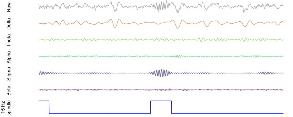
Finally, here is an example spindle detected in this individual, shown alongside the bandpass filtered EEG for delta, theta, alpha and beta power as well as sigma power. As expected (i.e. by definition), the spindle corresponds to a brief increase in sigma power:

Note

Primarily in the context of lunaR, in the near future we'll be adding tutorials and helper functions to facilitate automatically making these types of plots quickly for all spindles in a dataset.

Thresholds

The core of the spindle detection algorithm involves imposing discrete thresholds on the quantitative metrics derived from the continuously-varying EEG. As such, there are a lot of magic numbers inherent in the spindle detection process. One of the key parameters is the threshold which the normalized wavelet coefficient must exceed for a putative spindle to be scored (the default of which is 4.5 times the mean). But is 4.5 a good magic number? What about 2 instead? Or what about 20? And so on...

To get some insight into whether this may be an appropriate choice for the particular individuals and analyses under consideration, Luna has a set of functions that evaluate different thresholds based on Otsu's method, a technique from computer vision that attempts to set a threshold so as to minimize the within-class variance (and so correspondingly, maximize the between class variance) in the two classes that are formed by placing a dichotomizing threshold on a continuous measure. In our scenario, the measure is the wavelet coefficient, and we are trying to place a threshold that roughly corresponds to "spindle" and "non-spindle".

If the continuous metric exhibits clear bimodality, this approach should easily find a threshold that effectively splits the two peaks. In the context of spindles, where things are likely to be a bit messier, we consider the distribution of wavelet coefficients to be a mixture of two classes: the null distribution of noise, i.e. where there is no true spindle, and a second, less frequency class representing points where a spindle is present (and where we will expect higher values of the wavelet coefficient).

Parameters

Parameter	Example	Description
`empirical`	`empirical`	Empirically determine thresholds
`set-empirical`	`set-empirical`	Use empirically determined thresholds for spindle detection
`verbose-empirical`	`verbose-empirical`	Output extensive information on threshold estimation

Output

Individual-level output (option: empirical, strata: F x CH)

Variable	Description
`EMPTH`	Empirically-determined threshold
`EMPF`	Relative frequency of above-thresholds points based on `EMPTH`
`MEAN_OVER_MEDIAN`	Ratio of mean to median, to index skewness of the wavelet coefficients

Between-class variance over range of thresholds (option: empirical, strata: TH x F x CH)

Variable	Description
`SIGMAB`	Between-class variance for given threshold

Example

Here we use this approach on the three tutorial individuals: we run a basic command to estimate spindles (for all NREM2 sleep, with no other artifact detection in place), adding the empirical threshold:

luna s.lst sig=EEG -o out.db -s "MASK ifnot=NREM2 & RE & SPINDLES fc=11,15 empirical"

In lunaR, we use ldb() to load the resulting out.db file:

k <- ldb("out.db")

We extract the relevant table of results by different thresholds (TH):

d <- lx( k , "SPINDLES" , "CH_F_TH" )

As this table contains all three individuals, we'll use lid() and basic R functions to create three plots separately, of the between-class variance as a function of threshold, split by fast and slow spindles. First, we get a list of the individual IDs:

ids <- unique( d$ID )

Then we loop to create three plots:

par(mfcol=c(1,3))
for (id in ids) { 
t <- lid( d , id )  
plot( t$TH[ t$F==11 ] ,  t$SIGMAB[ t$F == 11 ] , 
      type="l" , lwd=2 , col="orange" , 
      main=id, xlab="Threshold" , ylab="Between-class variance" , ylim=c(0,1)) 
lines( t$TH[ t$F==15 ] ,  t$SIGMAB[ t$F == 15 ] , type="l" , lwd=2 , col="skyblue" ) 
legend( 5,0.2,c("11 Hz","15 Hz"),fill=c("orange","skyblue"))
}

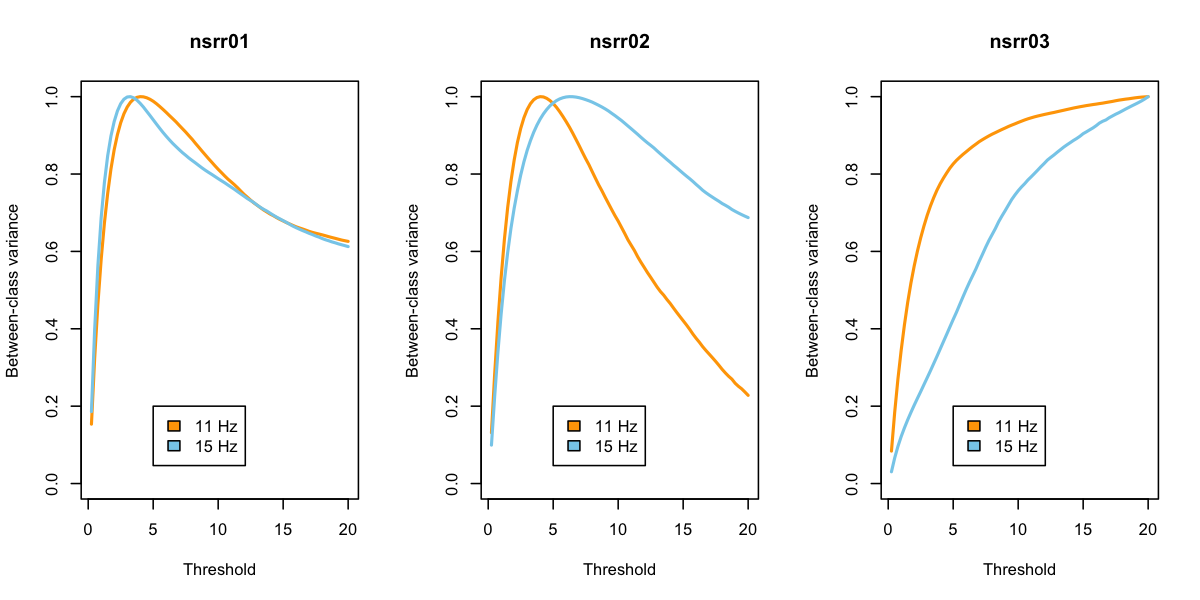
For the first two individuals, based on Otsu's criterion at least, this suggests that thresholds around 4 or 5 are optimal, in the sense of maximizing the between class variance (i.e. in wavelet coefficients between "spindle" and "non-spindle" classes). For the third individual, the results look strange, suggesting that extreme threshold such as 20 times the mean is optimal. This is mirrored in the individual-level output for EMPTH and EMPF: the optimal thresholds and the corresponding area under the curve:

destrat out.db +SPINDLES -r F CH -v EMPTH EMPF -p 3

ID       CH   F   EMPF   EMPTH
nsrr01   EEG  11  0.034  4.000
nsrr01   EEG  15  0.067  3.250
nsrr02   EEG  11  0.041  4.000
nsrr02   EEG  15  0.024  6.250
nsrr03   EEG  11  0.001  20.000
nsrr03   EEG  15  0.002  20.000

This suggests there may be something off with the EEG channel for nsrr03. As well as looking at the raw data, one approach may be to impose some automated artifact detection prior to spindle detection and threshold estimation (i.e. as we would typically recommend). Re-running with aberrant epochs removed prior to spindle detection (i.e. by including ARTIFACTS and SIGSTATS commands:

luna s.lst sig=EEG -o out2.db -s "MASK ifnot=NREM2 & RE \
                                  & ARTIFACTS mask & SIGSTATS mask th=3,3,3 & RE \
                                  & SPINDLES fc=11,15 empirical"

This appears to normalize the "optimal" thresholds somewhat, in that the area under the curve (i.e. roughly corresponding to the portion of time in "spindle" versus "non-spindle" states) are ball-park what we may expect to observe in a typical individual who has around 2 or so spindles per minute detected at a central scalp EEG channel, with each spindle lasting approximately 1 second (i.e. 2/60 = 0.033):

destrat out2.db +SPINDLES -r F CH -v EMPTH EMPF -p 3

ID      CH   F    EMPF    EMPTH
nsrr01  EEG  11   0.046   3.500
nsrr01  EEG  15   0.092   2.750
nsrr02  EEG  11   0.041   4.000
nsrr02  EEG  15   0.029   5.500
nsrr03  EEG  11   0.033   4.000
nsrr03  EEG  15   0.066   3.000

Returning to the plots, things look a bit better:

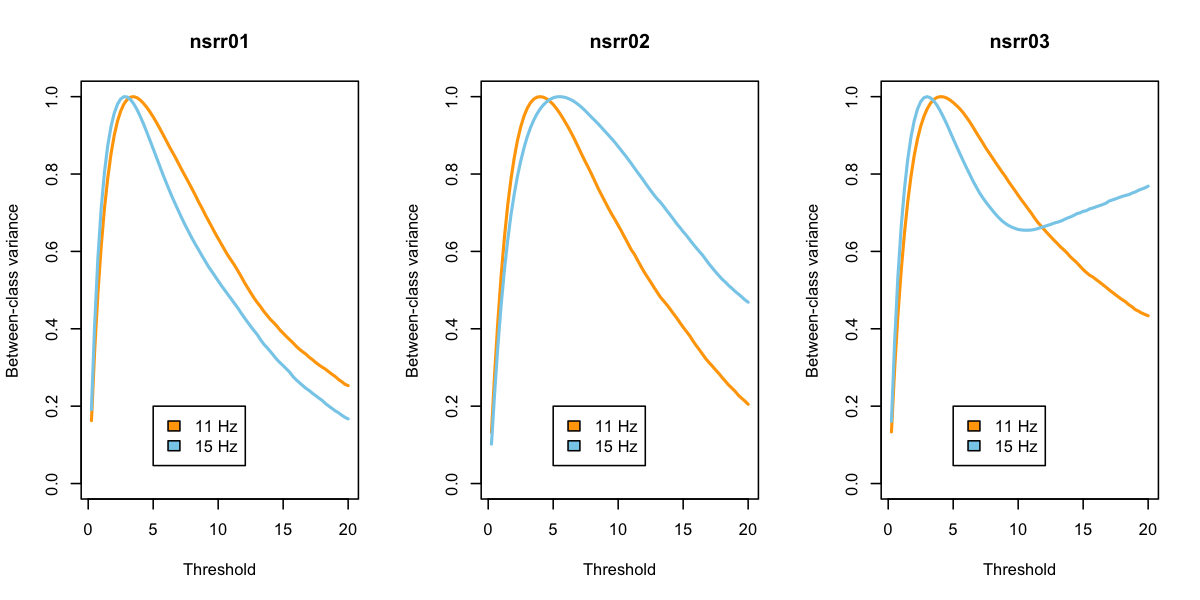
What to make of all this? We do not advise selecting different "optimal" thresholds for each individual based on these analyses. Rather, we suggest that looking at these (and other) metrics can be useful in basic sanity-checking for whether a given analysis for a given individual is likely to yield meaningful results.

Quality metrics

Luna calculates a simple QC metric for each spindle, by considering the relative increase of non-spindle activity within the spindle interval, relative to spindle-activity. We use five fixed bands, which unlike the PSD command, are not altered by changing special variables. The three non-spindle bands are: delta (0.5-4 Hz), theta (4-8 Hz), and beta (defined here as 20-30 Hz). The two spindle bands are slow sigma (10-13.5 Hz) and fast sigma (13.5-16 Hz).

For each channel, Luna calculates the baseline power for each band, P^band. For the interval spanning the i^th spindle, we calculate band power P_i^band. We then calculate relative enrichment for each band (on a log10 scale), as:

E_i^band = log10(P_i^band) - log10(P^band).

The Q score for each spindle is based on the difference between the largest spindle-band relative enrichment versus the largest non-spindle band relative enrichment:

Q_i = max( E_i^slow-sigma , E_i^fast-sigma ) - max( E_i^delta , E_i^theta , E_i^beta )

That is, numbers less than zero indicate that a non-spindle band is showing greater relative enrichment (relative to the baseline log-scaled power for that band) than either spindle band. Such spindles are more likely to reflect artifact which had a non-specific effect on the power spectrum.

To illustrate this QC metric, we'll detect spindles for the second tutorial individual:

luna s.lst 2 sig=EEG -o out.db \
  -s "MASK ifnot=NREM2 & RE & \
      SPINDLES fc=11,15 enrich q=-9 annot=sp1 cycles=12"

Here, we detect both fast and slow spindles, targeting 11 and 15 Hz respectively; we've set cycles to 12 instead of the default 7, in order to increase frequency-specificity. We've added the enrich option to output E_i^slow-sigma and E_i^fast-sigma along with E_i^delta E_i^theta and E_i^beta for each spindle/channel/target-frequency/band (and so stratified by CHxFxSPINDLExB). We also set q equal to -9, which effectively turns off any QC filtering, so that we can see what some spindles that would not otherwise have been called with the default threshold (q=0) look like. Finally, the ftr option writes out two files that detail where spindles occur.

In lunaR:

library(luna)
lattach( lsl( "s.lst" ) , 2 )

We'll attach as annotations the two newly-created files:

ladd.annot.file( "id_nsrr02_feature_SPINDLES-spindles-EEG-wavelet-11-sp1.ftr" ) 
ladd.annot.file( "id_nsrr02_feature_SPINDLES-spindles-EEG-wavelet-15-sp1.ftr" )

We'll then load our previously-generated results, saved in out.db:

k <- ldb( "out.db" )

and extract the table which contains Q_i, the per-spindle quality metric.

d <- lx( k , "SPINDLES" , "F" , "CH" , "SPINDLE" )

Plotting the distribution of this separately for slow and fast spindles:

par(mfcol=c(1,2))
hist( d$Q[ d$F == 11 ] , breaks=30 , main="11 Hz spindles" , xlab="Q" , xlim=c(-2,2) ) 
abline(v=0,col="red",lwd=2)
hist( d$Q[ d$F == 15 ] , breaks=30 , main="15 Hz spindles" , xlab="Q" , xlim=c(-2,2) )
abline(v=0,col="red",lwd=2)

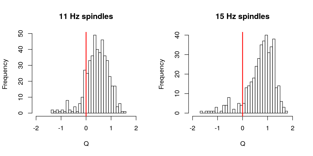
We see that most spindles (as would be expected) have quality scores greater than 0, meaning that the interval showed greater spindle-band enrichment than non-spindle-band enrichment.

Of the full set (i.e. running without the default q=0 threshold in place), we see that approximately 10% of spindles have q less than 0:

table( d$Q > 0 , d$F )

         11  15
  FALSE  68  36
  TRUE  405 370

Let's visualize some q<0 and q>0 spindles (we'll actually select qc>1 spindles, to ensure that we don't randomly select spindles with q very near 0). For simplicity, we'll do this just for fast spindles.

First, we'll save the labels of the two new annotation tracks we appended (i.e. you can see the names from running lannots()):

a15 = "SPINDLES-spindles-EEG-wavelet-15-sp1"

We'll then extract the intervals of each annotation instance, i.e. each spindle:

s15 <- lannots( a15 )

Confirming that we get 406 spindles, i.e. as output above, we can see length(s15) is indeed 406.

For visualization, here we'll just select five low Q and five high Q spindles:

lo15 <- sample(d$SPINDLE[ d$Q < 0 & d$F == 15 ])[1:5]
hi15 <- sample(d$SPINDLE[ d$Q > 1 & d$F == 15 ])[1:5]

Using lunaR functions, we can then write a function to plot the raw EEG signal for each spindle, with a 4-second flanking window on either side:

f1 <- function(i,a) { 
x <- ldata.intervals( i , chs = "EEG" , annots = a , w = 4 )
y <- x$EEG
plot( x$SEC , y , type="l" , axes=F,xlab="",ylab="" , ylim=c(-125,125) )
t <- x$SEC[ x[,lsanitize(a)] == 1 ]
points( t , rep( -125,length(t)) , col=rgb(0,0,255,150,max=255) , pch="|" )
}

Finally, we'll generate a matrix of plots, with the five low Q spindles in the left column, and the five high Q spindles in the right column:

par(mfrow=c(5,2),mar=c(0,0,0,0) )
for (i in 1:5) {
f1( i = s15[ lo15[ i ] ] , a = a15 )
f1( i = s15[ hi15[ i ] ] , a = a15 )
}

As you can see, the low Q spindles (that would not have been detected using Luna's default q=0 setting) appear to reflect some sources of artifact, whereas, as a whole, the high Q spindles look more like canonical spindles.

Be aware that setting q too high may unnecessarily miss many true spindles though. A value of q=0.3 (i.e. log10(2)) requires that the spindle-band enrichment is at least twice non-spindle band enrichment; a value of q=1 requires a 10-fold enrichment. Considering the distribution of mean Q over all individuals in the study may provide a good starting point, if you want to select non-default values.

Warning

Naturally, neither this particular automated spindle detection algorithm, nor this particular quality metric, are guaranteed to always get it right... We fully expect that this algorithm will flag as a "spindle" events that most scorers would not, and vice versa. When first approaching this tool, we'd advise experimenting with the different thresholds and parameters, and spot-check studies in the way we have above. (The lunaR tutorial shows how to automatically iterate through all spindles detected.)

In general, if visual review seems to indicate likely artifact, the spindle is likely to be a false positive. In contrast, however, otherwise high Q spindles may appear relatively modest on visual review, and may not have been detected by some human scorers. Human scoring does not constitute a real gold-standard, however, and both human and automatic approaches impose inherently arbitrary thresholds on what is likely a continuously-varying and heterogeneous set of physiological processes. As such, we'd advise against automatically assuming the automatic detector is wrong, at least for this latter class of events ("low amplitude spindles").

Overall, the usual principles of a) trying to ensure that high-quality data go into the analysis, and b) working with large samples and appropriate statistical techniques downstream, are likely to be just as (if not more) important than spending too much tweaking the detection procedure, or agonizing over what is or is not "a true spindle".

Collating spindles

When detecting spindles on multiple channels or at multiple, nearby frequencies, what presumably is the same underlying physiological event may often be detected multiple times. These options assist in collating the results of spindle detection across channels and/or frequencies:

you can control whether two temporally close spindles detected on the same channel/target-frequency should be merged and considered as one event or not (merge parameter, the default is 0.5 seconds)
second, within channel, you can collate temporally overlapping spindles detected at nearby frequencies (i.e. we would expect a great deal of overlap in the results of an analysis with F_C=10 Hz and F_C=11 Hz).
third, across channels, you can collate temporally overlapping spindles detected at nearby target frequencies; these may or may not represent physiologically distinct events depending on the montage and channels being collated.

These commands essentially take a list of spindles and generate another list of so-called m-spindles: groups of spindles that, on some definition, "overlap", i.e. represent the same underlying event.

The primary output from this analysis is an estimate of m-spindle density (MSP_DENS), i.e. which is taken to reflect the total number of unique spindles (i.e. allowing for potentially overlapping definitions). For each m-spindle (set a spindles), Luna also calculates an mean frequency (a weighted mean of the constituent spindle frequencies, with weights given by the ISA of each spindle). This is output for each spindle and also used to generate a frequency-conditioned estimate of m-spindle density.

Parameters

Parameter	Example	Description
`merge`	`merge=0.2`	Merge two putative spindles if within this interval (default 0.5 seconds)
`collate`	`collate`	Within each channel, collate overlapping spindles with similar frequencies (to `MSPINDLES`)
`collate-channels`	`collate-channels`	As above, except merge across channels also
`th-frq`	`th-frq=1`	Criterion for merging two spindles if difference in frequency is within this range (default 2 Hz)
`list-all-spindles`	`list-all-spindles`	List all spindles that comprise each m-spindle

Secondary parameters:

Parameter	Example	Description
`th-interval`	`th-interval=0.5`	Merge two overlapping spindles if the ratio of intersection to union is at least this value (default 0, i.e. any overlap)
`th-interval-cross-channel`
`th-interval-within-channel`
`window`	`window=0.5`	Set window around each spindle when defining temporal overlap
`hms`	`hms`	Show clock-time of each m-spindle

Output

Individual-level summaries of m-spindles (option: collate, strata: none)

Variable	Description
`MSP_DENS`	m-spindle density
`MSP_N`	m-spindle count
`MSP_MINS`	Denominator for density, i.e. minutes of signal analyzed

m-spindle density stratified by m-spindle frequency (option: collate, strata: F )

Variable	Description
`MSP_DENS`	m-spindle density conditional on m-spindle frequency

Merged-spindle output (option: collate, strata: MSPINDLE)

or Merged-spindle output (option: collate-within-channel, strata: CH x MSPINDLE)

Variable	Description
`MSP_DUR`	Duration of this m-spindle
`MSP_F`	Estimated frequency of this m-spindle
`MSP_FL`	Lower frequency of this m-spindle
`MSP_FU`	Upper frequency of this m-spindle
`MSP_SIZE`	Number of spindles in this m-spindle
`MSP_STAT`	Statistic for m-spindle
`MSP_START`	Start time (seconds elapsed from EDF start) of m-spindle
`MSP_STOP`	Stop time (seconds elapsed from EDF start) of m-spindle

Spindle to m-spindle mappings (option: list-all-spindles, strata: SPINDLE x MSPINDLE)

Variable	Description
`SCH`	Spindle label (channel:target frequency)
`FFT`	Spindle estimated frequency (via FFT)
`START`	Spindle start time (elapsed seconds from EDF start)
`STOP`	Spindle stop time (elapsed seconds from EDF start)

Additional output (option: hms, strata: MSPINDLE or CH x MSPINDLE))

Variable	Description
`MSP_START_HMS`	Merged spindle start clock-time
`MSP_STOP_HMS`	Merged spindle stop clock-time

Example

luna s.lst 2 sig=EEG -o out.db -s "MASK ifnot=NREM2 & RE & \
                                   SPINDLES fc-lower=10 fc-upper=16 fc-step=0.25 \
                                            collate list-all-spindles"

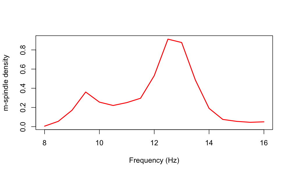
The total m-spindle density is 4.89 spindles per second, i.e. this estimates the total unique number of spindles over this broad frequency range ( with target frequencies of 10-16 Hz and each wavelet spanning approximately plus/minus 2 Hz):

destrat out.db +SPINDLES

ID       MSP_DENS   MSP_MINS    MSP_N
nsrr02   4.8972     199.5       977

We can also view the m-spindle density as a function of the estimated m-spindle frequency: i.e. these numbers will sum to the total MSP_DENS estimate (or close to it, as we only consider the fixed range of 8 to 16 Hz in 0.5 Hz bins, by default, when outputing this):

destrat out.db +SPINDLES -r F

Plotting the output of this command, we potentially see evidence of a bimodality in spindle frequencies for this individual:

Relationship to individualized spindle detectors

Rather than using fixed target frequencies (e.g. 13.5 Hz, 11 Hz, or 15 Hz, etc) to define "spindles", some approaches to spindle detection seek to find, empirically, the "peak" or "peaks" (which may or may not be obviously present in the power spectra) for each particular individual, and then target spindles of those particular frequencies for that individual. In contrast, this approach is effectively agnostic to an individual's "true" characteristic spindle frequency (or frequencies), or to having to define spindle frequencies up front, by virtue of simply considering all possible frequencies in the broad sigma range, and then combining results. (Arguably this approach might be preferred a priori in any case, on the grounds that even within a single individual we can see marked shifts in spindle frequency over the course of the night.)

Other metrics

The following options report some additional spindle morphology characteristics (these are unlikely to be desired as part of any primary spindle analysis, and so can be ignored by most users). The if option estimates spindle instantaneous frequency, averaged over spindles, as a function of the relative location within the spindle. The tlock option produces an averaged EEG signature of detected spindles, synced to the spindle peak (point of max peak-to-peak amplitude).

Parameters

Parameter	Example	Description
`if`	`if`	Estimate instantaneous frequency of spindles
`if-frq`	`if-frq=1`	Window around target frequency (default 2 hz)
`if-emp-frq`	`if-emp-frq=1`	Window around observed frequency (default 2 hz)
`tlock`	`tlock`	Flag to request (verbose) average, peak-locked waveforms

Instantaneous frequency is estimated via the filter-Hilbert method, where the filter is F_C +/- H Hz (where H is set by if-frq, default 2). Using if-emp-frq over if-frq is typically more robust and is preferred, however.

Output

Instantaneous frequency (IF) per spindle (option: if, strata: CH x F x SPINDLE)

Variable	Description
`IF`	Mean frequency per spindle over duration

Mean IF stratified by relative location in spindle (option: if, strata CH x F x RELLOC)

Variable	Description
`IF`	Mean frequency of all spindles, per relative position within the spindle (five bins)

Example

With the tutorial data:

luna s.lst 2 -o out.db -s "MASK ifnot=NREM2 & RE & \
                           SPINDLES sig=EEG fc=11,15 if tlock q=0.3 cycles=12"

To get the estimate of IF per spindle (which will should typically be very highly correlated with FRQ and FFT, as they are all estimating essentially the same thing):

destrat out.db +SPINDLES -r F CH SPINDLE -v FFT FRQ IF

To get the mean IF stratified by relative position with the spindle (i.e. dividing each spindle into five, equally-sized time bins):

destrat out.db +SPINDLES -r F CH RELLOC -p 3

ID  CH  F   RELLOC  IF
nsrr02  EEG 11  1   11.321
nsrr02  EEG 11  2   11.218
nsrr02  EEG 11  3   11.041
nsrr02  EEG 11  4   10.912
nsrr02  EEG 11  5   10.818
nsrr02  EEG 15  1   14.287
nsrr02  EEG 15  2   14.119
nsrr02  EEG 15  3   13.959
nsrr02  EEG 15  4   14.015
nsrr02  EEG 15  5   14.181

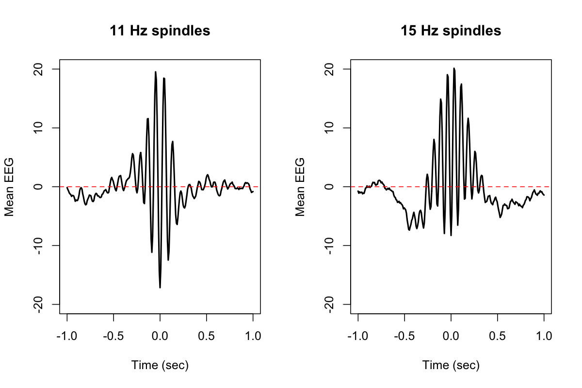
To plot the mean signal time-locked to each spindle peak (in lunaR):

k <- ldb("out.db")

d <- lx( k , "SPINDLES" , "CH" , "F" , "MSEC" ) 

par( mfcol=c(1,2) )
for (f in c(11,15)) { 
 plot( d$MSEC[ d$F==f ] , d$TLOCK[ d$F==f ] , ylim=c(-20,20) , type="l"
       xlab="Time (sec)",ylab="Mean EEG",main=paste(f,"Hz spindles"), lwd=2)
 abline(h=0,col="red",lty=2)
}

Annotations

Luna can generate annotation files representing the spindles detected in a given run. These can be output (e.g. with WRITE-ANNOTS) and subsequently be attached to an EDF via lunaR, for example, in order to visualize spindles, as in the examples above.

Parameters

Parameter	Example	Description
`annot`	`s1`	Add an annotation to the in-memory dataset

Output

The annot option generates annotations with the class ID as specified by annot. The instance ID will be set to the target frequency; the annotation channel ID will be set to the appropriate channel.

SPINDLES sig=C3,C4 fc=11,15 annot=sp1 & WRITE-ANNOTS file=sp1.annot

# sp1 | Spindle intervals
class   instance   channel  start        stop         meta
sp1     15         C3       11861.797    11862.469    .
sp1     15         C4       11861.852    11862.531    .
sp1     15         C3       11866.898    11867.664    .
sp1     11         C3       11876.195    11876.984    .
sp1     11         C4       11876.195    11877.062    .
...

Spindle/SO coupling

Adding the so option for the SPINDLES command instructs Luna to detect slow oscillations and report on their temporal coupling with spindles. In short, Luna lines up the phase of slow oscillations with the "peaks" of spindles (the point of maximal peak-to-peak amplitude, typically near the center of the spindle), and then estimates the mean SO angle across spindle peaks, and two metrics of that measure the strength of non-random temporal coupling between SO and spindles.

Either all spindles all are included in this analysis (if the all-spindles option is given), or only spindles that overlap a detected SO (the default). In the former case, Luna will still use the SO phase whether or not it would have explicitly reported a SO spanning that spindle.

A magnitude metric (MAG) is calculated based on the intra-trial phase clustering (ITPC) statistic for all spindles, or those overlapping a detected SO. Second, an overlap metric (OVERLAP) is calculated, reflecting the proportion of spindles that show any overlap (temporally) with a SO (for that same channel). This second, overlap metric is not reported if all-spindles is given.

If nreps is specified, Luna will perform that number of randomized analyses, based on datasets in which spindle peaks are shuffled under the null hypothesis of no specific coupling between spindles and SO. The behavior of the permutation can be changed, such that instead of spindles being shuffled only within the spanning epoch (the default), they are shuffled across all epochs (perm-whole-trace). Here, the entire set of spindle peaks is shifted by a constant (wrapping around the end/start of the signal, as necessary). Second, if all-spindles option is not specified, then when evaluating the magnitude of coupling, spindles are shuffled (each independently) only within the spanning SO (again, wrapping as necessary). That is, in this latter case, each null replicate contains exactly the same number of spindles and slow oscillations, the same number of which show overlap in each replicate. The only thing that is randomized in this scenario is the precise temporal association with spindle peak and SO phase within detected SOs.

Parameters

For the primary parameters of the SO detection heuristic, see the section on the SO command below. These include:

frequency band (f-lwr, f-upr, etc)
amplitude criteria (mag, uV-neg, uV-p2p, etc)
duration criteria (t-lwr, t-upr, etc)

In addition to the above, the so option of the SPINDLES command has additional parameters for the analysis of spindle/SO coupling:

Parameter	Example	Description
`nreps`	`nreps=10000`	Number of shuffled/surrogate time-series to generate
`all-spindles`		Consider all spindles, whether or not they overlap a SO
`perm-whole-trace`		Do not use within-epoch shuffling
`stratify-by-phase`		Additional overlap statistics per 20-degree SO phase bin

Output

The so option of the SPINDLES command produces the same set of outputs as the SO command (see below), describing the number and properties of the detected SOs. In addition, the so option of the SPINDLES command generates extra outputs describing the temporal coupling between spindles and SOs, described here:

Primary individual-level spindle/SO coupling output (option: so, strata: CH x F)

Variable	Description
`COUPL_MAG`	Magnitude of coupling (ITPC metric)
`COUPL_OVERLAP`	Number of spindles overlapping a detected SO
`COUPL_ANGLE`	Circular mean of SO phase at spindle peak (`SO_SPHASE_PEAK` below)
`COUPL_PV`	Asymptotic p-value for the ITPC statistic

Permutation-based spindle/SO coupling output (options: so, nreps, strata: CH x F)

Variable	Description
`COUPL_MAG_Z`	Z score for `COUPL_MAG` based on surrogate time series
`COUPL_MAG_NULL`	Mean coupling magnitude under the null
`COUPL_MAG_EMP`	Empirical p-value for `COUPL_MAG` based on surrogate time series
`COUPL_OVERLAP_NULL`	Mean overlap under the null
`COUPL_OVERLAP_Z`	Z-score for `COUPL_OVERLAP`
`COUPL_OVERLAP_EMP`	Empirical p-value for `COUPL_OVERLAP`
`COUPL_SIGPV_NULL`	Rate of null replicates with a p<0.05 significant asymptotic ITPC

Spindle-level spindle/SO coupling output (option: so, strata: CH x F x SPINDLE)

Variable	Description
`SO_SPHASE_PEAK`	SO phase at spindle peak
`NEAREST_SO`	Time to nearest SO
`NEAREST_SO_NUM`	Number of nearest SO

SO morphology (option: so verbose-coupling, strata: CH x PHASE)

Variable	Description
`SOPL_EEG`	Phase-locked mean EEG value (as a function of SO phase, in 20-deg bins)

SO morphology (option: so verbose-coupling, strata: CH x SP)

Variable	Description
`SOTL_EEG`	Time-locked mean EEG value (as a function of sample-points before/after SO negative peak)

Spindle/SO phase coupling (option: so verbose-coupling, strata: CH x F x PHASE)

Variable	Description
`SOPL_CWT`	SO-phased locked mean spindle wavelet coefficient (18 20-deg bins)

Spindle/SO phase coupling (option: so verbose-coupling, strata: CH x F x SP)

Variable	Description
`SOTL_CWT`	Time-locked mean spindle wavelet coefficient

Example

Here we consider spindle/SO coupling for the second individual from the tutorial data. We'll only consider NREM2 sleep, for fast (15 Hz target frequency) and slow (11 Hz target frequency) at default settings. We achieve this by adding so to the SPINDLES command, along with the definition of the SO (see below). Here we'll use a relative/adaptive threshold of 1.5 times the baseline mean, along with othe default settings (e.g. for the duration and frequency of the SO).

luna s.lst nsrr02 -o out.db -s 'MASK ifnot=NREM2 & RE & SPINDLES fc=11,15 sig=EEG so mag=1.5'

As seen from the log/console, Luna now also detected slow oscillations (as the SO command would do):

 detecting slow waves: 0.2-4.5Hz
  - relative threshold 1.5x median
  - full waves, based on consecutive positive-to-negative zero-crossings
 25380 zero crossings, of which 4977 met criteria (thresholds (<x, >p2p) -14.7917 30.0472)
 running Hilbert transform

You can see information about the number and properties of detected SOs as follows (nb. not all output shown):

destrat out.db +SPINDLES -r CH | behead

                       ID   nsrr02              
                       CH   EEG                 
                       SO   4977                
                   SO_AMP   -27.9675273648175   
                   SO_DUR   0.686249547920436   
                   SO_P2P   47.9202863568751    
                  SO_RATE   24.9473684210526

That is, 4977 SO were detected, or 24.9 per minute (SO_RATE), with an average duration of 0.69 seconds (SO_DUR) i.e. around 1.4 Hz. Note these are based on NREM2 sleep only, and this definition of SO is quite liberal, i.e. most of NREM2 is determined as having a "slow oscillation" under this particular definition, and on average the SO only has a negative deflection of -28uV. See below for alternate definitions.

In terms of coupling between the SO and spindles, we can look at the output table stratified by spindle target frequency (F) and channel (CH):

destrat out.db +SPINDLES -r F CH | behead

Here are the relevant results for slow spindles:

              COUPL_ANGLE   324.240526870805    
                COUPL_MAG   0.133073212508123   
                 COUPL_PV   0.206789334851279   
            COUPL_OVERLAP   89                  
                        N   249

Here are the same metrics for fast spindles:

              COUPL_ANGLE   267.757606950599    
                COUPL_MAG   0.456849609921408   
                 COUPL_PV   2.04211688177307e-13
            COUPL_OVERLAP   140                 
                        N   393

Based on the asymptotic p-values (COUPL_PV), we see highly significant spindle/SO coupling for fast but not slow spindles in this individual. 140 (of 393) fast spindles overlap a detected SO. For fast spindles, the mean SO phase angle at spindle peaks is 267 degrees. SO phase angle is defined starting from a positive-to-negative zero-crossing, as follows:

Location	Phase angle
Positive-to-negative zero-crossing	0/360 degrees
Negative peak	90 degrees
Negative-to-positive zero-crossing	180 degrees
Positive peak	270 degrees

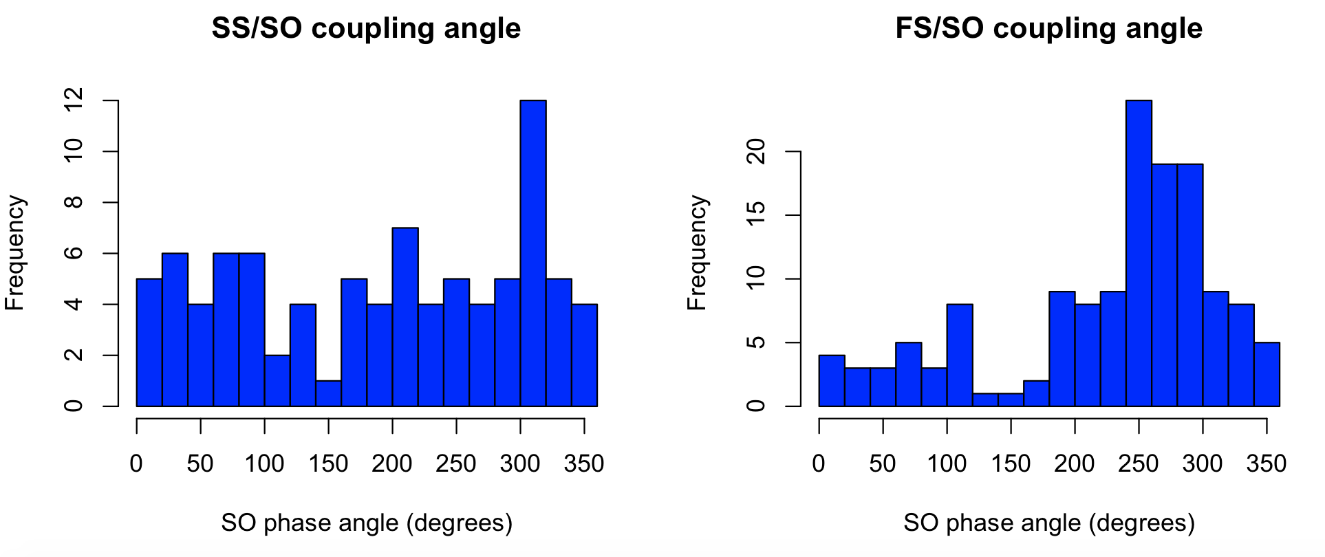
We can also see, for each spindle, whether or not the spindle overlapped a SO, and if so, the SO phase angle:

destrat out.db +SPINDLES -r F CH SPINDLE -v SO_PHASE_PEAK > o.txt

Looking at the results in R:

d <- read.table("o.txt",header=T)

We see that fast spindles (FS) preferentially have their peak around the positive peak (270 degrees) of SO. In contrast, the pattern is less clear for slow spindles (SS) in this particular individual/analysis:

par(mfcol=c(1,2))
hist( d$SO_PHASE_PEAK[ d$F == 11  ] , breaks=15 , col = "blue" , xlab="SO phase angle (degrees)" , main="SS/SO coupling angle" ) 
hist( d$SO_PHASE_PEAK[ d$F == 15  ] , breaks=15 , col = "blue" , xlab="SO phase angle (degrees)" , main="FS/SO coupling angle" )

Next, we'll add random shuffling to the coupling analyses, to generate empirical, non-parametric estimates of significance, by adding the nreps command. Here we specify 100,000 random permutations per analysis (these are evaluated quite quickly), running now only for fast spindles:

luna s.lst nsrr02 -o out.db \
      -s 'MASK ifnot=NREM2 & RE \
          & SPINDLES fc=15 sig=EEG so mag=1.5 nreps=100000'

We now see some additional metrics in the output. For example, whereas as observed 140 spindles overlapping a SO (COUPL_OVERLAP), we see that on average, in each null replicate, only 104.2 spindles overlapped a SO (COUPL_OVERLAP_NULL). Based on these statistics, this gives an empirical p-value of 0.028 (COUPL_OVERLAP_EMP), i.e. in this individual, we see significant (p<0.05) overlap between spindles and SO at the gross level:

destrat out.db +SPINDLES -r F CH  | behead

              COUPL_ANGLE   267.757606950599    
                COUPL_MAG   0.456849609921408   
            COUPL_MAG_EMP   9.99990000099999e-06
           COUPL_MAG_NULL   0.105944405707361   
              COUPL_MAG_Z   7.14893183381634    
            COUPL_OVERLAP   140                 
        COUPL_OVERLAP_EMP   0.027649723502765   
       COUPL_OVERLAP_NULL   104.1836            
          COUPL_OVERLAP_Z   2.22339252291559    
                 COUPL_PV   2.04211688177307e-13
         COUPL_SIGPV_NULL   0.2081

The corresponding values for the ITPC metric are 0.46 observed (COUPL_MAG) versus an average of 0.11 (COUPL_MAG_NULL) under the null, giving an empirical p-value of 9.9e-6. Note: this is the smallest possible empirical p-value if only 100,000 replicates are specified, i.e. 1/(1+100000).

Note

As they are based on randomization, naturally, you may get numerically slightly different values for some of these metrics, if you repeat the above analysis on the tutorial data.)

Note that COUPL_SIGPV_NULL shows that over 20% of null-replicates had an asymptotic ITPC p-value significant at the p<0.05 level. That this is approximately four times greater than we'd expect by chance suggests that the asymptotic p-values are, in this situation, anti-conservative (i.e. we'd expect a 5% rate to be p<0.05 under the null). The observed 2e-13 asymptotic p-value is therefore likely to be inflated too. These considerations motivate the use of empirical p-values in this context, given known biases with the ITPC (and similar) metrics. That is, prefer to use COUPL_MAG_EMP or COUPL_MAG_Z as measures of spindle/SO coupling strength, rather than COUPL_MAG or COUPL_PV.

Next, we can run the same analysis, but adding the all-spindles option to extend the coupling analysis to all spindles, i.e. whether or not they overlap a detected SO:

luna s.lst nsrr02 -o out2.db -s 'MASK ifnot=NREM2 & RE & SPINDLES fc=15 sig=EEG so mag=1.5 nreps=100000 all-spindles'

Now the COUPL_OVERLAP metrics are not shown, i.e. as this analysis ignores whether or not a particular SO was detected; rather the estimated instantaneous phase from the Hilbert transform of the slow-wave band-pass filtered signal is used irrespective:

              COUPL_ANGLE   249.957585228371    
                COUPL_MAG   0.23828160431191    
            COUPL_MAG_EMP   0.010469895301047   
           COUPL_MAG_NULL   0.0555142478440371  
              COUPL_MAG_Z   4.60828305383158    
                 COUPL_PV   2.03816238295918e-10
         COUPL_SIGPV_NULL   0.13594             
                        N   393

Here we see an attenuated but still significant spindle/SO coupling (i.e. COUPL_MAG_EMP is 0.01). In this example, however, using the larger number of spindles (i.e. all 393 here, rather than only the 140 SO-overlapping ones) does not appear to give stronger results (although, not the asymptotic p-values are high in each case).

Verbose coupling output

The verbose-coupling option, along with so, produces some additional tables/output strata that can be used to generate plots describing the nature of spindle/SO coupling:

luna s.lst nsrr02 -o out.db -s 'MASK ifnot=NREM2 & RE & SPINDLES fc=15 sig=EEG so mag=1.5 nreps=100000 verbose-coupling'

Four additional strata are added to the output:

  [SPINDLES]    : CH PHASE          : 18 level(s)   : SOPL_EEG
                :                   :               : 
  [SPINDLES]    : CH SP             : 251 level(s)  : SOTL_EEG

  [SPINDLES]    : F CH PHASE        : 18 level(s)   : SOPL_CWT
                :                   :               : 
  [SPINDLES]    : F CH SP           : 251 level(s)  : SOTL_CWT

The first two contain the average EEG, either as a function of SO phase, or time-locked to the negative peak of each SO. The second two contain the average spindle wavelet power (and so are dependent on F, the target frequency for the spindle analysis too). For example, we can extract and use R to plot SOPL_EEG and SOPL_CWT, the SO phase-locked raw EEG and spindle CWT respectively:

par(mfcol=c(1,2))
plot( d$PHASE , d$SOPL_CWT , type="b" , xlab="SO phase angle (degrees)" , ylab="CWT coefficient" , pch=20  ) 
plot( d$PHASE , d$SOPL_EEG , type="b" , xlab="SO phase angle (degrees)" , ylab="Mean raw EEG (uV)" , pch=20  )

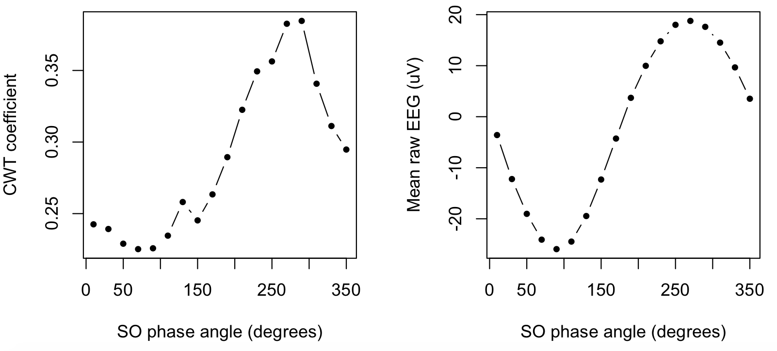
That is, the right panel confirms (as expected/defined) the typical SO, which has a positive peak at 270 degrees. The left panel shows how the spindle wavelet power (i.e. the underlying metric upon which spindles are explicitly detected) also has a peak that corresponds to the SO positive peak.

Second, we can request additional COUPL_OVERLAP output, where rather than assessing any overlap between a spindle and a SO, here we instead count overlap between a spindle and a particular point of a SO, defined by SO phase (in 18 bins each of 20 degrees). That is, we add the stratify-by-phase option:

luna s.lst nsrr02 -o out.db -s 'MASK ifnot=NREM2 & RE & SPINDLES fc=15 sig=EEG so mag=1.5 nreps=100000 stratify-by-phase'

This has the effect of generating an additional table/output strata, defined by F and PHASE for a given channel (CH):

  [SPINDLES]    : F CH PHASE        : 18 level(s)   : COUPL_OVERLAP COUPL_OVERLAP_EMP
                :                   :               : COUPL_OVERLAP_Z

The definitions of the COUPL_OVERLAP metrics are as above, except now they are conditional on SO-phase bin.

destrat out.db +SPINDLES -r F CH PHASE

ID       CH    F    PHASE  COUPL_OVERLAP  COUPL_OVERLAP_EMP   COUPL_OVERLAP_Z
nsrr02   EEG   15   10     4               0.934              -1.235
nsrr02   EEG   15   30     3               0.958              -1.378  
nsrr02   EEG   15   50     3               0.958              -1.384  
nsrr02   EEG   15   70     5               0.794              -0.637  
nsrr02   EEG   15   90     3               0.981              -1.676  
nsrr02   EEG   15   110    8               0.440               0.287   
nsrr02   EEG   15   130    1               1.000              -2.450  
nsrr02   EEG   15   150    1               1.000              -2.587  
nsrr02   EEG   15   170    2               0.996              -2.047  
nsrr02   EEG   15   190    9               0.447               0.261   
nsrr02   EEG   15   210    8               0.642              -0.230  
nsrr02   EEG   15   230    9               0.516               0.084   
nsrr02   EEG   15   250    24              0.000               5.147   
nsrr02   EEG   15   270    19              0.005               2.968   
nsrr02   EEG   15   290    19              0.002               3.344   
nsrr02   EEG   15   310    9               0.355               0.508   
nsrr02   EEG   15   330    8               0.458               0.241   
nsrr02   EEG   15   350    5               0.810              -0.685

That is, COUPL_OVERLAP still adds to 140, as in the above example, but these spindles are now listed depending on exactly when in the SO the spindle peak lies. Plotting these metrics in R:

par(mfrow=c(2,2))
plot( d$PHASE , d$COUPL_OVERLAP , pch=20 , type="b" , xlab="SO phase angle (degrees)" , ylab="N spindles overlapping SO" )
plot( d$PHASE , d$COUPL_OVERLAP_Z , pch=20 , type="b" , xlab="SO phase angle (degrees)" , ylab="Z statistic" )
plot( d$PHASE , d$COUPL_OVERLAP_EMP , pch=20 , type="b" , xlab="SO phase angle (degrees)" , ylab="Empirical p-value" )
plot( d$PHASE , -log10(d$COUPL_OVERLAP_EMP ), pch=20 , type="b" , xlab="SO phase angle (degrees)" , ylab="-log10(empirical p-value)" )
abline( h=-log10( 0.05) , lty=2)

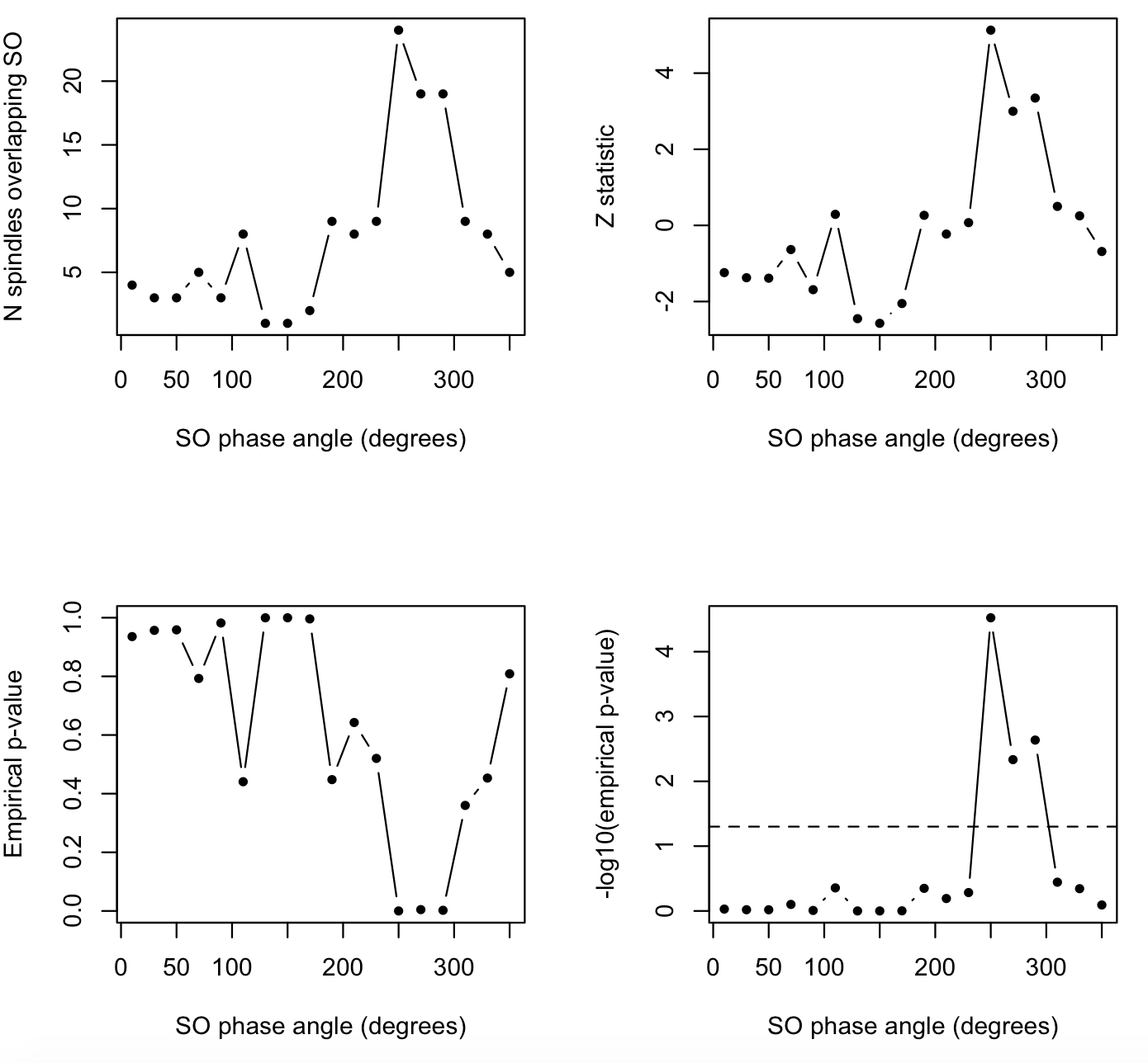
That is, we see the above-chance rate of spindle/SO overlap is not uniformly distributed across the entire, but is concentrated around 250-290 degrees (consistent with the significant COUPL_MAG which is another way to tell us the same thing).

See the SO section below for more details on how to define slow oscillations.

Misc

show-coef

The show-coef is primarily for development purposes and should not be part of a standard spindle-analysis workflow. It produces a lot of output: five values for every time-point for every channel for every spindle frequency: this will be hard work for the output database, which is not really designed for this type of data: you are better off using this without the -o database option; rather, extract the desired information directly from standard output:

luna s.lst 1 < cmd.txt \
  | awk ' $2 == "SPINDLES" && $5 == "CWT" { print $3,$4,$6 } ' OFS="\t"

Variable	Description
`RAWCWT`	Absolute, raw wavelet coefficient value
`CWT`	Normalized wavelet coefficient value
`CWT_TH`	Wavelet threshold for core spindle
`CWT_TH2`	Wavelet threshold for flanking spindle
`CWT_THMAX`	Wavelet max threshold for spindle

SO

Detects slow oscillations via a simple, heuristic approach

The SO command uses an heuristic approach to detect slow oscillations (SO) in the sleep EEG, combined with filter-Hilbert estimation of SO phase. This command can also be invoked through the so parameter of SPINDLES command, in which case additional metrics describing spindle/SO coupling are also reported.

The SO command works by first bandpass-filtering the EEG (given the frequency parameters) and then applies a series of time and amplitude criteria to identify individual SOs. Either absolute (fixed) or adaptive (relative) amplitude thresholds can be specified.

Parameters

The example section below illustrates the application of these parameters, which determine what constitutes a detected SO.

Bandpass filtering prior to SO detection:

Parameter	Example	Description
`f-lwr`	`f-lwr=0.2`	Bandpass filter lower transition frequency
`f-upr`	`f-upr=4.5`	Bandpass filter upper transition frequency

Time criteria for SO detection:

Parameter	Example	Description
`t-lwr`	`t-lwr=`	Minimum duration of a SO
`t-upr`	`t-upr=`	Maximum duration of a SO
`t-neg-lwr`	`t-neg-lwr=0.5`	Lower threshold for negative peak (seconds)
`t-neg-upr`	`t-neg-lwr=2`	Upper threshold for negative peak (seconds)

Amplitude criteria for SO detection:

Parameter	Example	Description
`mag`	`mag=1`	Use a relative amplitude threshold instead (see below)
`uV-neg`	`uV-neg=-75`	Negative peak amplitude threshold ( default 0, i.e. no threshold )
`uV-p2p`	`uV-p2p=140`	Peak-to-peak amplitude (default 0, i.e. no threshold)
`th-mean`	`th-mean`	Use mean (instead of median) for thresholding
`stats-median`	`stats-median`	Use median (instead of mean) for reporting SO stats (not for epoch-level reports)

Additional options;

Parameter	Example	Description
`tl`	`tl=sig1,sig2`	Other signals to be summarized w.r.t. time-locked SO
`onset`	`onset`	Time-lock to SO onset instead of negative peak
`pos`	`pos`	Time-lock to SO positive peak instead of negative peak
`window`	`window=1`	Window around SO peak (default +/- 3 seconds)

Outputs

Primary SO information per channel (strata: CH)

Variable	Description
`SO`	Number of SO detected
`SO_RATE`	SO per minute
`SO_AMP`	Median amplitude (of negative peak)
`SO_P2P`	Median peak-to-peak amplitude
`SO_DUR`	Median SO duration
`SO_SLOPE`	Median slope (by default, `SO_SLOPE_NEG2`
additional metrics w/ `verbose`:
`SO_SLOPE_NEG2`	Median slope (negative peak to negative-to-positive zero-crossing)
`SO_NEG_DUR`	Median negative peak duration
`SO_POS_DUR`	Median positive peak duration
`SO_SLOPE_NEG1`	Median slope (positive-to-negative zero-crossing to negative peak)
`SO_SLOPE_POS1`	Median slope (negative-to-positive zero crossing to positive peak)
`SO_SLOPE_POS2`	Median slope (positive peak to positive-to-negative zero-crossing)
`SO_TH_NEG`	Threshold used for negative peak
`SO_TH_P2P`	Threshold used for peak-to-peak

Per SO output (strata: CH x N)

Variable	Description
`START`	Start of SO (in seconds elapsed from start of EDF)
`STOP`	Stop of SO (in seconds elapsed from start of EDF)
`DUR`	SO duration
`UP_AMP`	SO positive peak amplitude
`DOWN_AMP`	SO negative peak amplitude
`P2P_AMP`	SO peak-to-peak amplitude
`SLOPE_NEG2`	Slope (upward slope of negative peak)
additional metrics:
`START_IDX`	Sample index of SO start
`STOP_IDX`	Sample index of SO stop
`UP_IDX`	Sample index of positive peak
`DOWN_IDX`	Sample index of negative peak
`SLOPE_POS1`	Slope (alternate metric)
`SLOPE_POS2`	Slope (alternate metric)
`SLOPE_NEG1`	Slope (alternate metric)

Epoch-level counts of SO (strata: CH x E)

Variable	Description
`N`	Number of SOs detected in that epoch

Time-locked signal averaging (option: tl, strata: CH x CH2 x SP)

Variable	Description
`SOTL`	Average signal for `CH2`, time-locked by SO detected in `CH`

Example

The SO detection routine operates as follows:

Band-pass filter the signal with transition frequencies f-lwr and f-upr (defaulting to 0.5 and 4 Hz)
Find all positive-to-negative zero-crossings in the filtered signal
Retain intervals between consecutive zero-crossings that are between t-lwr and t-upr in duration (defaulting to 0.8 and 2.0 seconds)
Either apply absolute amplitude filtering, designating SO as intervals with a negative peak below uV-neg (e.g. if uV-neg=-75 this means more negative, i.e. -80 uV ) and a peak-to-peak amplitude greater than uV-p2p
Or apply adaptive amplitude filtering, designing SO as intervals with negative peak of mag times the median (or mean, if th-mean) negative peak and a peak-to-peak amplitude mag times the median (or mean, if th-mean) peak-to-peak amplitude; the thresholds are written to the output (SO_TH_NEG and SO_TH_P2P)

As an example, looking at N3 sleep in the second individual from the tutorial dataset, for the first EEG channel (EEG), and using an adaptive threshold with a factor of 2 times the median:

luna s.lst nsrr02 -o out.db -s 'MASK ifnot=NREM3 & RE & SO sig=EEG mag=2'

 detecting slow waves: 0.2-4.5Hz
  - relative threshold 2x median
  - full waves, based on consecutive positive-to-negative zero-crossings
 9418 zero crossings, of which 824 met criteria (thresholds (<x, >p2p) -34.1888 69.5302)
 running Hilbert transform

Looking at the primary output variables:

destrat out.db +SO -r CH | behead

                       SO   824                 
                   SO_AMP   -51.3357345906725   
                   SO_DUR   1.0331359223301     
                   SO_P2P   89.7069054223203    
                  SO_RATE   8.90810810810811

We see there were 824 SOs detected, or a rate of 8.9 per minute. On average, each SO was 1.03 seconds long, had a negative peak amplitude of -51.3uV, and a peak-to-peak amplitude of 89.7uV.

In the literature, different investigators have used different definitions for SOs in different contexts. Instead of using a relative amplitude threshold (mag), you could set an absolute threshold. For example, here we require a negative peak of at least -40 uV, and at least 75 uV peak-to-peak:

luna s.lst nsrr02 -o out.db 
                  -s 'MASK ifnot=NREM3 & RE & SO sig=EEG uV-neg=-40 uV-p2p=75'

                       SO   555                 
                   SO_AMP   -56.1938081995994   
                   SO_DUR   1.04608288288288    
                   SO_P2P   96.1411853282356    
                  SO_RATE   6

Alternatively, here we require even larger waveforms:

luna s.lst nsrr02 -o out.db 
                  -s 'MASK ifnot=NREM3 & RE & SO sig=EEG uV-neg=-75 uV-p2p=140'

                       SO   13                  
                   SO_AMP   -94.4252281038546   
                   SO_DUR   1.08553846153846    
                   SO_P2P   168.084348953554    
                  SO_RATE   0.140540540540541

Naturally, the amplitude is larger here, but there are far fewer SOs (here fewer than one per minute).

Hint

It is also possible to specify time limits for the positive and negative components separately:

t-neg-lwr=0.3 t-neg-upr=1.5  t-pos-lwr=0.0 t-pos-upr=1.0

Here we combine all definitions in a single command, this time for N2 and N3 sleep combined, using TAG to organize the results (by adding a tag R). We'll also generate data to visualize the average waveforms, using tl:

luna s.lst nsrr02 -o out.db 
      -s 'MASK all & MASK unmask-if=NREM2,NREM3 & RE & 
          TAG R/1 & SO sig=EEG mag=2 tl=EEG window=2 & 
          TAG R/2 & SO sig=EEG uV-neg=-40 uV-p2p=75 tl=EEG window=2 & 
          TAG R/3 & SO sig=EEG uV-neg=-75 uV-p2p=140 tl=EEG window=2 '

Looking at the SO rate for each threshold definition, we recover the above values:

destrat out.db +SO -r R CH -v SO_RATE SO

ID       CH    R   SO     SO_RATE
nsrr02   EEG   1   4304   14.74
nsrr02   EEG   2   896    3.07
nsrr02   EEG   3   25     0.086

Now we see a larger difference in the estimated SO rate between the first two methods (R of 1 and 2), reflecting that fact that adding N2 sleep effectively lowers the threshold for detecting SOs, leading to an overall higher rate, which may at first be counter-intuitive. In contrast, for the two absolute definitions, the average rate lowers when considering N2 and N3 combined versus just N3 sleep.

Extracting information from the tl option, this gives the averaged EEG signal time-locked to the negative SO peak:

destrat out.db +SO -r R CH CH2 SP > d.txt

we can load this into R and plot it:

d <- read.table("d.txt",header=T)
plot( d$SP[d$R==1], d$SOTL[d$R==1] , type="l" , col="blue" , lwd = 2 , 
      ylim = c(-100 , 50 ) , 
      xlab="Time from negative SO peak (sample-points)" , ylab="Signal" ) 
lines( d$SP[d$R==2], d$SOTL[d$R==2] , col="red" , lwd = 2 )
lines( d$SP[d$R==3], d$SOTL[d$R==3] , col="green" , lwd = 2 )

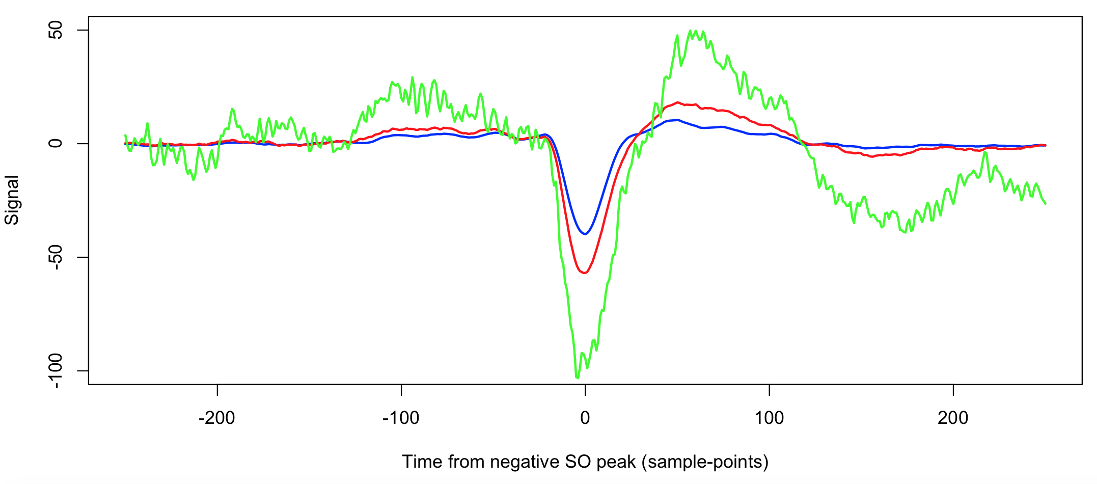
The three methods 1, 2 and 3 are blue, red and green respectively. The green line (R3) is more variable as a smaller number of SO were averaged over. Otherwise, we see that the second method (red line) yields slightly longer SOs of slightly greater amplitude.

Depending on the study population (e.g. children versus elderly, or mice versus human), and depending on the purpose of the analysis, different approaches may give better results. For example, estimating spindle/SO coupling will not be possible if there are not a sufficient absolute number of SOs (and/or spindles) in the recording.

luna s.lst nsrr02 -o out.db -s 'MASK all & MASK unmask-if=NREM2,NREM3 & RE & 
     TAG R/1 & SPINDLES so fc=15 sig=EEG mag=2                 nreps=1000000 verbose-coupling & 
     TAG R/2 & SPINDLES so fc=15 sig=EEG uV-neg=-40 uV-p2p=75  nreps=1000000 verbose-coupling & 
     TAG R/3 & SPINDLES so fc=15 sig=EEG uV-neg=-75 uV-p2p=140 nreps=1000000 verbose-coupling '

destrat out.db +SPINDLES -r R CH F -v COUPL_OVERLAP COUPL_MAG_Z COUPL_OVERLAP_Z | behead

                       ID   nsrr02              
                       CH   EEG                 
                        F   15                  
                        R   1                   
              COUPL_MAG_Z   9.2884209252313     
            COUPL_OVERLAP   115                 
          COUPL_OVERLAP_Z   2.99092347889109    

                       ID   nsrr02              
                       CH   EEG                 
                        F   15                  
                        R   2                   
              COUPL_MAG_Z   6.49847282659681    
            COUPL_OVERLAP   54                  
          COUPL_OVERLAP_Z   4.7739523530548     

                       ID   nsrr02              
                       CH   EEG                 
                        F   15                  
                        R   3                   
              COUPL_MAG_Z   0                   
            COUPL_OVERLAP   1                   
          COUPL_OVERLAP_Z   0.770177278950557

Here we see greater evidence for non-random the magnitude of spindle/SO coupling (based on the empirical distribution of the ITPC statistic) under the first method (Z=9.2 for R1 versus Z=6.5 for R2), likely due to the greater number of observations. The third method (R3) only detects a couple of SOs in the dataset, with only a single instance of spindle/SO overlap (COUPL_OVERLAP is 1). In terms of gross overlap, R2 is slightly more power than R1 in this instance (Z=4.8 for R2 versus Z=3.0 for R1).

destrat out.db +SPINDLES -r R F CH PHASE > d.txt

d <- read.table("d.txt",header=T)
plot( d$PHASE[d$R==1], d$SOPL_CWT[d$R==1], 
      type="l" , lwd=2, col="blue" , ylim=c(0,0.6) , 
      xlab="SO phase (0/360 is positive-to-negative zero-crossing)" , 
      ylab="Spindle wavelet power") 
lines( d$PHASE[d$R==2], d$SOPL_CWT[d$R==2] , lwd=2, col="red" ) 
abline(v=270,lty=2)

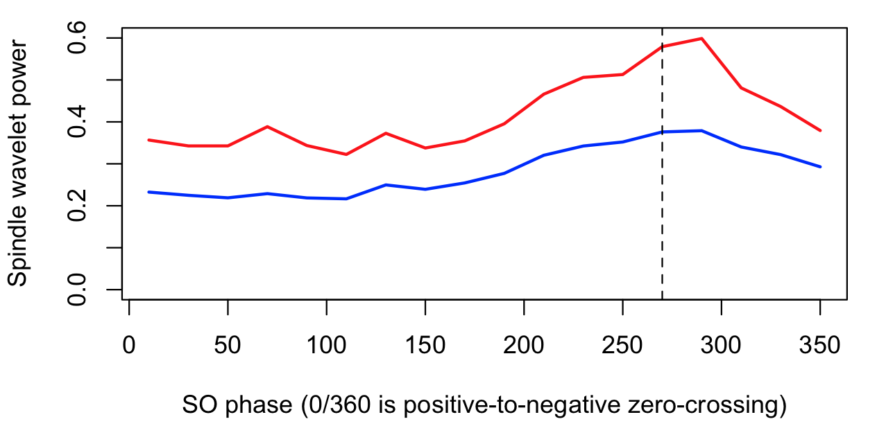
Here we see, for both R1 and R2 definitions, an increased fast spindle wavelet power around the negative peak of the SO (270 degrees) for this individual.