Artifact detection

Commands to perform artifact detection/correction

Command	Description
`CHEP-MASK`	CHannel/EPoch (CHEP) outlier detection
`ARTIFACTS`	Per-epoch Buckelmueller et al. (2006) artifact detection
`LINE-DENOISE`	Line denoising via spectrum interpolation
`SUPPRESS-ECG`	Correct cardiac artifact based on ECG
`ALTER`	Reference-channel regression-based artifact correction
`EDGER`	Utility to flag likely artifactual leading/trailing intervals

CHEP-MASK

Epoch-wise Hjorth parameters and other statistics

CHEP masks indicate whether particular CHannel/EPoch pairs are unusual or likely artifacts. As explained in this vignette, the CHEP-MASK is designed to work hand-in-hand with CHEP and potentially (in the context of hdEEG sleep data) INTERPOLATE commands.

This command calculates and reports per-epoch Hjorth parameters and (optionally) other statistics: signal root mean square (RMS), indices of signal clipping (the proportion of points that equal the minimum or maximum for that epoch), absolute maximum absolute values and flatness (proportion of points of a similar value to the preceding value).

Luna will mask channel/epoch pairs (called cheps here) that are (statistical) outliers (i.e. potentially indicative of signal artifacts) for these measures. For Hjorth parameters, thresholds for outlier detection can be set iteratively: for example, first, to flag epochs more than 2 standard deviations (SD) from the mean, and then second, to flag more epochs that are more than 2 SDs from the mean based on the epochs that survived round 1, etc. This iterative heuristic can be useful if some epochs are outliers by many orders of magnitude, as those can effectively hide other epochs that are less pronounced but outliers nonetheless.

A few notes on using CHEP-MASK to detect outlying epochs:

CHEP-MASK respects previously set CHEP masks and does not include them in the outlier detection process, i.e. as they have already been removed. To alter this behavior use ep-th0, ch-th0 and chep-th0 options in place of ep-th, ch-th and chep-th (described below).
You can set a smaller epoch size such as EPOCH len=4 for finer-grained artifact detection.
As well as Hjorth parameters, CHEP-MASK can flag epochs based on the proportion of sample points in a given epoch that are a) above a certain absolute value (max), that are clipped (clipped) or flat (flat).

Parameters

Core parameters:

Parameter	Example	Description
`sig`	`sig=C3,F3`	Restrict analysis to these channels
`ep-th`	`ep-th=3,3`	SD-unit threshold(s) for Hjorth within-channel/between-epoch outlier detection
`ch-th`	`ch-th=2`	SD-unit threshold(s) for Hjorth between-channel/within-epoch outlier detection
`chep-th`	`chep-th=5`	SD-unit threshold(s) for Hjorth general outlier detection

Additional options:

Parameter	Example	Description
`clipped`	`clipped=0.05`	Flag epochs with this proportion of clipped sample points
`flat`	`flat=0.05`	Flag epochs with this proportion of flat sample points (optionally `flat=0.05,1e-4`)
`max`	`max=200,0.05`	Flag epochs with this proportion of points with absolute value above 200

Output

The CHEP-MASK command only alters the CHEP mask and writes some information to the console. No other output is generated. Use the CHEP command following CHEP-MASK to produce summary statistics on the number of epochs/channels masked, etc.

Example

See this vignette for an application of CHEP-MASK to hdEEG data.

Here, we'll consider a simpler application in the context of a PSG recording with only two central EEG channels. Taking the first individual from the tutorial, here we calculate epoch-level metrics for the first EEG channel, and flag outliers that are greater than 2 standard deviations from the mean (performed twice, iteratively).

luna s.lst 1 sig=EEG -o out.db -s 'CHEP-MASK sig=EEG ep-th=2,2 '

 CMD #1: CHEP-MASK
   options: ep-th=2,2 sig=EEG
  set epochs to default 30 seconds, 1364 epochs
  within-channel/between-epoch outlier detection, ep-th = 2,2
   iteration 1: removed 261 channel/epoch pairs this iteration (261 in total)
   iteration 2: removed 115 channel/epoch pairs this iteration (376 in total)

By itself, CHEP-MASK only alters the internal CHEP mask: to actually remove these potentially aberrant epochs, we need to pair this commadn with CHEP, which sets the epoch-level mask based on the current CHEP mask:

luna s.lst 1 sig=EEG -o out.db -s ' CHEP-MASK sig=EEG ep-th=2,2
                                  & CHEP epochs
                                  & DUMP-MASK
                                  & RE '

Here we see output from CHEP which shows that we are now dropping those flagged epochs, by setting the epoch-level mask:

 CMD #2: CHEP
   options: epochs=T sig=EEG
  masking epochs with >0% masked channels: 376 epochs
  CHEP summary:
   376 of 1364 channel/epoch pairs masked (28%)
   376 of 1364 epochs with 1+ masked channel, 376 with all channels masked
   1 of 1 channels with 1+ masked epoch, 0 with all epochs masked

Finally, the RESTRUCTURE (or RE) takes the epoch-level mask and actually drops those epochs permanently from the internal representation of the data - i.e. any subsequent analysis would be based on this subset of 988 epochs, not the full set.

 CMD #3: RE
   options: sig=EEG
  restructuring as an EDF+:   keeping 29640 records of 40920, resetting mask
  retaining 988 epochs

The intervening DUMP-MASK command outputs the current state of the epoch-level mask (as used below).

The reason for separating out the steps of flagging channel/epoch pairs as outliers (CHEP-MASK), to setting particular epochs as outliers (for all channels, via CHEP), to actually removing the flagged epochs (with RE) is that it provides more flexibility to design artifact detection workflows that are suitable to different types of data/different modes of artifact.

Finally, the see the underlying Hjorth statistics used in the outlier detection, you would need to use the SIGSTATS command:

luna s.lst 1 sig=EEG -o hjorth.db -s 'SIGSTATS sig=EEG epoch'

We first extract epoch-level output (i.e. stratified by E as well as CH) into a plain-text file stats.txt:

destrat hjorth.db +SIGSTATS -r CH E > stats.txt

We can also pull the epochs actually masked, from the above run: destrat out.db +DUMP-MASK -r E > masked.txt Both these files have 1364 rows (plus a header), corresponding to the number of epochs in the original data. We can then use a package such as R to load and plot these data. For example, from the R command line:

d <- read.table( "stats.txt", header = T )
m <- read.table( "masked.txt", header = T )

head(d)

      ID  CH E        H1        H2       H3
1 nsrr01 EEG 1  98.45154 0.4807507 1.105732
2 nsrr01 EEG 2 234.34135 0.3164355 1.152268
3 nsrr01 EEG 3 159.33651 0.3511658 1.089591
4 nsrr01 EEG 4 181.39586 0.6554725 1.115427

Below, still using R, we plot four epoch-level metrics (H1 (log-scaled), H2 and H3), with the epochs set as outliers in purple:

f <- function(x) { ifelse(x,"purple","darkgray") } 
par(mfcol=c(3,1), mar=c(3,4,1,2) )
plot(d$E,log(d$H1) ,pch=20,cex=0.8,col=f(m$EMASK),xlab="Epoch",ylab="H1")
plot(d$E,d$H2      ,pch=20,cex=0.8,col=f(m$EMASK),xlab="Epoch",ylab="H2")
plot(d$E,d$H3      ,pch=20,cex=0.8,col=f(m$EMASK),xlab="Epoch",ylab="H3")

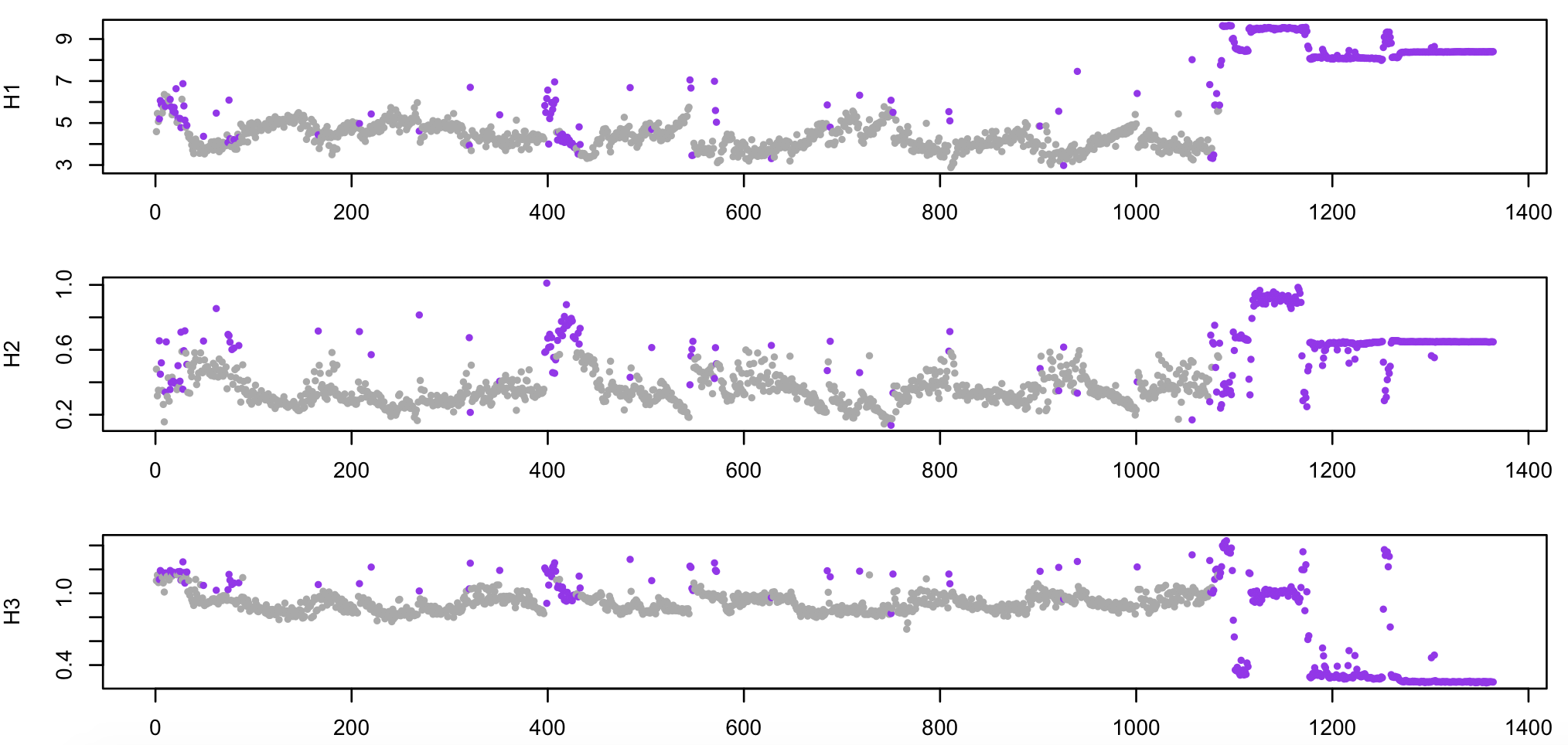
As noted above, all epochs past epoch 1100 or so are wake, essentially containing nothing but noise (e.g. if recording continued after electrodes were removed from the scalp). As expected, these have been flagged as likely artifact.

ARTIFACTS

Applies an artifact detection algorithm for EEG data

This command applies the method described in Buckelmueller et al, to detect likely artifacts in an EEG channel. Briefly, the method takes 10 4-second windows for each 30-second epoch to estimates delta (0.6 to 4.6 Hz) and beta (40-60Hz) spectral power, using Welch's method. Based on a sliding window of 15 epochs (i.e. seven either side of each epoch), an epoch is flagged to be masked if either the delta power is more than 2.5 times the local average (from the sliding window) or the beta power is more than 2.0 times the local average.

Parameters

Parameter	Example	Description
`sig`	`sig=C3,F3`	Restrict analysis to these channels
`verbose`	`verbose`	Report epoch-level statistics
`no-mask`	`no-mask`	Run, but do not set any masks

Output

Channel-level output (strata: CH):

Variable	Description
`FLAGGED_EPOCHS`	Number of epochs failing Buckelmueller
`ALTERED_EPOCHS`	Number of epochs actually masked
`TOTAL_EPOCHS`	Number of epochs tested

Epoch-level output (option: verbose, strata: CH x E):

Variable	Description
`DELTA`	Delta power
`DELTA_AVG`	Local average delta power
`DELTA_FAC`	Relative delta power factor
`BETA`	Beta power
`BETA_AVG`	Local average beta power
`BETA_FAC`	Relative beta power factor
`DELTA_MASK`	Masked based on delta power?
`BETA_MASK`	Masked based on beta power?
`MASK`	Whether the epoch is masked

Example

Taking the same EEG channel from the first tutorial EDF as in the SIGSTATS example above:

luna s.lst 1 sig=EEG -o out.db -s "ARTIFACTS verbose"

We see this command flags 60 epochs as potentially containing artifact:

masked 60 of 1364 epochs, altering 60

We can extract the epoch-level statistics from this analysis:

destrat out.db +ARTIFACTS -r E CH > d.txt

We can then use R to show the results, for delta (left column) and beta (right column) separately, showing log-scaled power per epoch (top row), the local average (middle row) and the epoch/local relative factor (bottom row), where purple points indicate that epoch was flagged as an outlier (by either delta or beta criterion).

d <- read.table("d.txt",header=T)
par(mfcol=c(3,2), mar=c(4,4,2,2) )
plot( log(d$DELTA)     , type="l" , ylab="Delta avg" )
plot( log(d$DELTA_AVG) , type="l" , ylab="Delta local")
plot( d$DELTA_FAC , pch=20 , col = f( d$MASK ) , ylab="Beta fac") 
plot( log(d$BETA)     , type="l" , ylab="Beta avg" )
plot( log(d$BETA_AVG) , type="l" , ylab="Beta local")
plot( d$BETA_FAC , pch=20 , col = f( d$MASK ) , ylab="Beta fac")

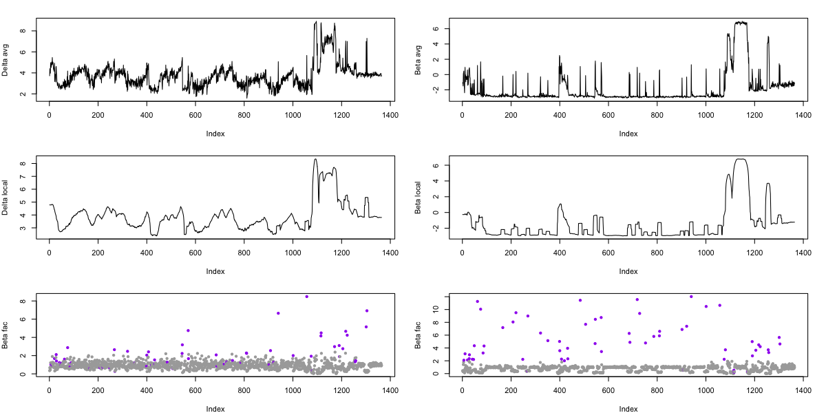
Comparing the results to the SIGSTATS method described above, which is applied to the same data, we see that this approach does a good job of flagging individual epochs with unusual artifacts, but does not flag the very extended stretches of gross artifact towards the end of the recording (i.e. because the entire local window is itself aberrant) . This latter type of artifact is, of course, easier to spot by eye, and is flagged by SIGSTATS. In practice, running multiple artifact detection/correction routines is usually warranted.

LINE-DENOISE

Attempt to attenuate electrical line noise at fixed frequencies, via spectrum interpolation

This command implements a spectrum interpolation approch to correcting certain types of line noise in EEG or other signals, following the approach described here.

Briefly, this approach works as follows:

obtain the amplitude spectrum via FFT
for fixed frequency windows, interpolate amplitude with mean of flanking regions
with phases unchanged, use Euler’s formula to obtain complex Fourier spectrum but with modified amplitudes
apply the inverse FFT to obtain a corrected time-domain signal

Parameters

Parameter	Example	Description
`sig`	`${eeg}`	Specify which signals to apply this method to
`f`	`20,40,60`	One or more target frequencies to set to missing and interpolate
`w`	`1,0.5`	Bandwidth of noise and neighbour intervals

Output

No output, just modifies the internal signals.

Example

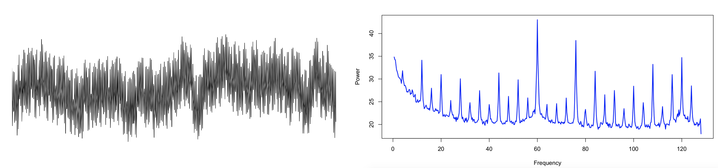
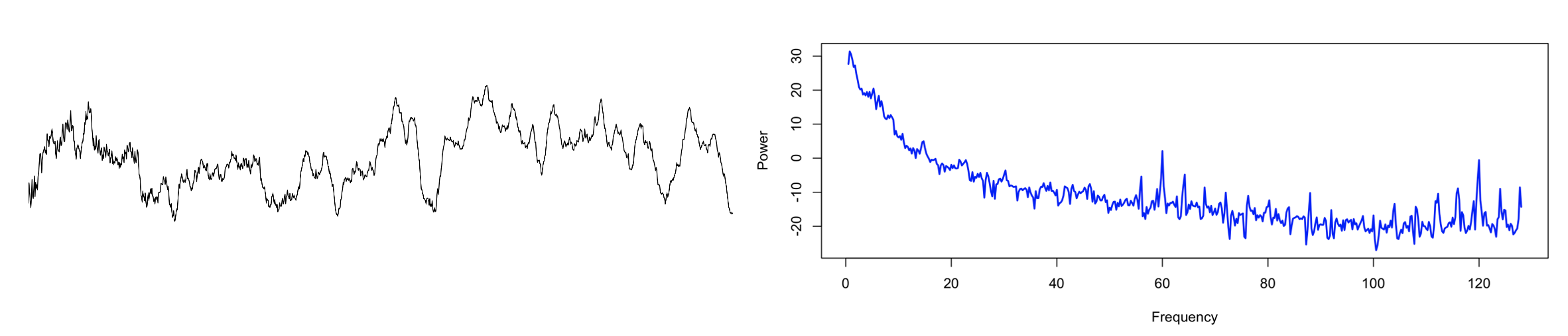
Here is one example recording with considerable line noise: the raw signal (left panel) for a single epoch, and the equivalent frequency spectrum up to 128 Hz (right panel). As well as line noise at 60 Hz, there are clear sub-harmonics at 4 Hz intervals, from which extend down into the regions typically considered of high physiological relevance for the sleep EEG, i.e. < 20 Hz.

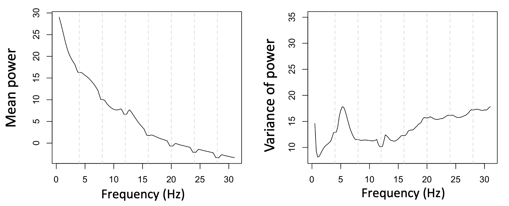
Zooming into the <25 Hz range, here we see the mean PSD for the entire sample (in this case, hundreds of individuals, many of whom turn out to share the same signature of electrical line noise, as was evident when looking at the full sample-level spectra up to 128 Hz):

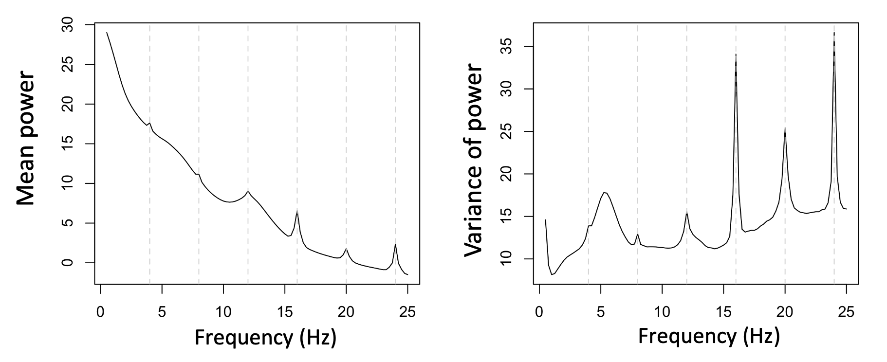
Although the impact on sample-level mean power in this frequency range is not extreme, in terms of individual differences, we see a clear and disturbing pattern, whereby the presence or absence of line-noise seems to drive clear spikes in the variance of power, and these seem to overwhelm physiological sources of between-individual variation. Naturally, this represents a rather large source of potential confounding.

We can apply the LINE-DENOISE approach to this sample, as follows (showing here just targetted frequencies up to 24 Hz); (nb. normally, one would add other commands, e.g. PSD or WRITE out new EDFs after running LINE-DENOISE):

luna s.lst –s LINE-DENOISE sig=${eeg} f=4,8,12,16,20,24 w=1,0.5

Warning

In this particular case, we observed relatively clear fixed-frequency artifacts across many individuals: naturally, in different samples, different individuals (or different portions of the recording) may show different patterns, and so this simple, one-size-fits-all approach may not be optimal.

In this particular case, this simple approach to removing line noise works quite well on this one individual:

Perhaps more significantly, when looking at the whole sample (i.e. applying the above to all individuals in this sample), we see a flatter mean PSD, but also greatly reduced variance at these 4 Hz intervals, suggesting that we've done a reasonable job at removing individual differences in power due to individual differences in the extent of line noise (e.g. especially at 16 Hz). Note that the mean PSD does show a few 'notches' suggesting that it has over-corrected in some cases.

Warning

Correcting the EEG signal in this manner naturally entails changing the data in a complex way, which partially attenuates the suspected artifactual signal sources, but potentially also induces subtle (or not so subtle) new confounds. Some downstream analyses may be more or less sensitive to these issues, and so these corrections may or may not be necessary or desirable. All steps here must be performed with care (using different approaches, or compared to the raw data, and checking for convergence with respect to the final, substantive results, if restricting analyses to clean data is not an option).

SUPPRESS-ECG

Given an ECG channel, detect R peaks and subtract cardiac-related contamination from the EEG

This command applies a modified Pan-Tompkins algorithm to detect QRS in the ECG. Based on the detected R-peaks, it estimates the average signature for other channels based on 2-second intervals time-locked with each R-peak. This is subtracted from the EEG, as described here. It also estimates heart rate per-epoch, and flags values likely to represent artifact. If needed, channels will be resampled to have similar sampling rates (to be set to the value of the parameter sr).

Parameters

Parameter	Example	Description
`ecg`	`ecg=ECG`	Specify which channel is the ECG
`sr`	`sr=125`	Set the sample rate that all channels should to resampled to
`no-suppress`	`no-suppress`	Run the command but do not alter any EEG channels

Output

Individual-level summaries (strata: none):

Variable	Description
`BPM`	Mean heart rate (bpm)
`BPM_L95`	Lower 95% confidence interval for mean HR
`BPM_U95`	Upper 95% confidence interval for mean HR
`BPM_N_REMOVED`	Number of epochs flagged as having invalid HR estimates
`BPM_PCT_REMOVED`	Proportion of epochs flagged as having invalid HR estimates

Epoch-level metrics (strata: E):

Variable	Description
`BPM`	Heart rate for this epoch (bpm)
`BPM_MASK`	Was this epoch invalid?

Channel-level summaries (strata: CH):

Variable	Description
`ART_RMS`	Root mean square of correction signature

Details of artifact signature (strata: CH x SP)

Variable	Description
`ART`	For each sample point in a 2-second window, the estimated correction factor

Example

Here we look at individual nsrr02 from the tutorial data, to identify and remove possible cardiac contamination in the EEG:

luna s.lst nsrr02 sig=EEG,ECG -o out.db < cmd.txt

The command file cmd.txt restricts analysis to NREM2 sleep, estimates EEG/ECG coherence (and spectral power), then estimates and corrects for cardiac contamination in the EEG, and finally, repeats the coherence and spectral analyses:

MASK ifnot=NREM2 
RE 
TAG R/pre 
COH 
PSD spectrum 
SUPPRESS-ECG ecg=ECG 
TAG R/post 
PSD spectrum 
COH

Hint

Note how we've used the TAG command to structure the output, by adding a factor R to denote whether the coherence and spectral analysis was performed pre or post the SUPPRESS-ECG command.

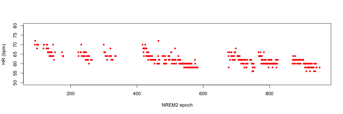
We can extract the per-epoch estimates of heart rate (bpm) and plot as follows:

destrat out.db +SUPPRESS-ECG -r R E > hr.txt

Plotting the BPM field of hr.txt against epoch (E), e.g. in R:

plot(d$E,d$BPM,pch=20,col="red",ylim=c(50,80),ylab="HR (bpm)",xlab="NREM2 epoch")

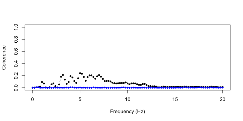
Second, we can extract the estimates of coherence between EEG and ECG as follows:

destrat out.db +COH -r F -c R -r CHS -v COH > d.txt

Plotting the pre (black) and post (blue) coherence values, for frequencies up to 20 Hz, we see that a non-trivial association between ECG and EEG channels has effectively been removed based on these metrics:

plot( d$F , d$COH.R.pre , ylim=c(0,1) , type="b" , pch=20, ylab="Coherence" , xlab="Frequency (Hz)" ) 
points( d$F , d$COH.R.post , ylim=c(0,1) , type="b" , pch=20, col="blue" )

Note, this is only a rough-and-ready approach to working with ECG data, which is not a primary focus of Luna. Other artifacts may well remain (e.g. in higher frequencies) and this approach may not work well with other datasets. That is, as usual, your mileage may vary...

Hint

When comparing different individual or signals, the ART_RMS metric can be taken as an approximate guide to the relative extent of contamination. The actual signatures (i.e. the R-peak sync'ed averaged EEG) can be viewed by looking at the ART variable, which is a channel by sample-point (CH x SP) metric.

ALTER

Simple regression-based or EMD approaches to handle certain artifacts

This command runs in one or two modes:

using explicit signals in the EDF as correctors (corr), i.e. proxies of any artifact in the target (sig) channel(s), and regressing out those components, following the approach outlined here. By default, the correction is performed in 5 second segments, as a sliding window with increment 2.5 seconds (i.e. 50% overlap). The final signal is based on weighted combinations of the overlapping estimates, to avoid edge artifacts in the reconstructed signal.
alternatively, applying EMD to the target (sig) channel, and subtracting components that are highly correlated with any of the corrector channels; or, if emd-corr option is present, also performing EMD on each corrector channel and removing any sig components that are highly correlated with one or more of the corrector (corr) components.

By default, the regression-based approach uses segments of 5 seconds, with 2.5 second overlap. The EMD-based approach uses non-overlapping 30-second segments. For now, we suggest using the regression-based mode of ALTER.

All sample rates must be similar for sig and corr channels.

Note

This command is explicitly called ALTER rather than CORRECT or some such... That is, depending on the the nature of the signals and the artifact, there is no guarantee that this approach will correctly remove the true, underlying sources of artifact.

Paramters

Option	Example	Description
`sig`	`C3`	Signal to be altered
`corr`	`LOC,ROC`	Signals to be used as references (i.e. proxies of artifact)
`segment-sec`	10	Segment size (default: 5 seconds for regression mode, 30 seconds for EMD mode)

For the EMD-based method, there are the following additional parameters:

Option	Example	Description
`emd`	`10`	Use EMD components of `sig` as references (instead of `corr` channels)
`th`	`0.9`	EMD-channel correlation threshold (default: 0.9)
`emd-corr`		Perform EMD on corrector signals (`corr`) also

Output

No output is generated, other than the in-memory channels specified by sig being altered.

Examples

We'll use a combination of real and simulated data to show how the ALTER command works. Note that, in practice, real artifacts (complex phenomena not necessarily well-captured by any one channel or component) are much more likely to be difficult to correct. That is, the performance in this toy dataset is not likely to be indicative of how well it performs on real data, e.g. with EMG, EOG or ECG artifact in the EEG.

We'll take 10 minutes of N2 data from a random study:

luna cfs.lst 1 -s ' MASK ifnot=N2
                    RE
                    REFERENCE sig=C3 ref=M2
                    SIGNALS keep=C3
                    MASK random=20 & RE
                    WRITE force-edf edf-dir=tmp '

We'll use the SIMUL command to spike in an artifactual signal (a simple sine wave) into the real EEG signal. Below, we'll call the original signal S1; the artifact is X1; the contaminated signal is S2 = S1 + X1; the cleaned signal is S3, which is intended to have the component due to X1 removed. That is, we run S3 (which is S1 plus X1) through the ALTER command, to see whether it removes this simple source of artifact:

luna tmp/file.edf -o out.db alias="S1|C3" \
  -s ' SIMUL sig=X1 frq=25 psd=2 sr=128
       TRANS sig=S2 expr=" S2 = S1 + X1 "
       TRANS sig=S3 expr=" S3 = S2 "
       ALTER sig=S3 corr=X1       
       COH spectrum max=50 
       PSD spectrum max=50 dB '

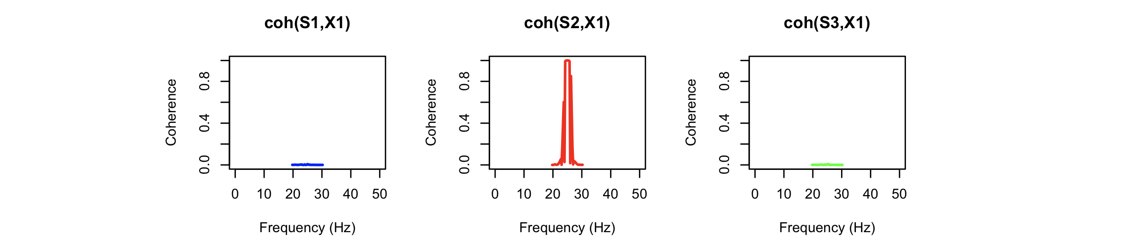
After running ALTER, we run COH and PSD to generate power spectra and coherence statistics for all signals. Here are the resulting power spectra:

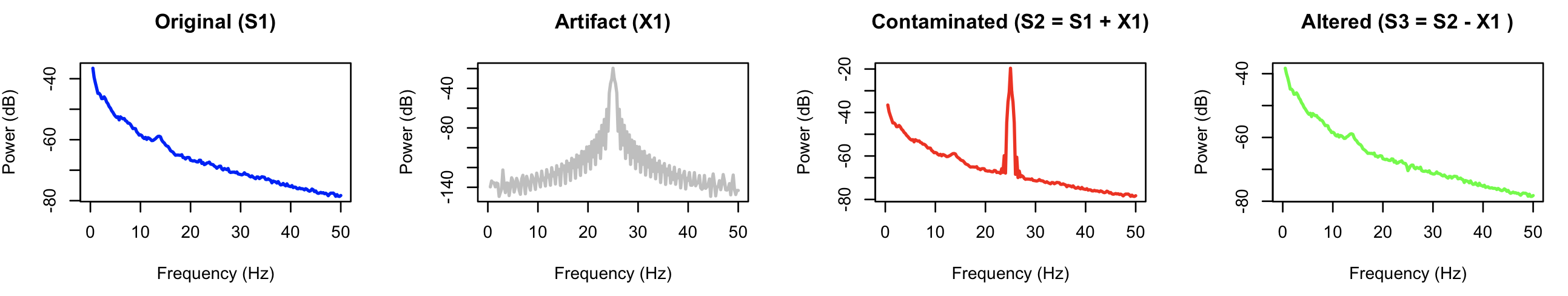
The final signal (S3) has clearly had the major source of artifact removed (versus the contaminated S2 signal), and shows a spectrum that is effectively identical to the original signal, S1.

Looking at the coherence statistics from COH, we see a very strong source of contamination around 25 Hz, which is the frequency of the simulated X1 artifact signal. This has effectively been completely removed in the altered signal (cohernece between S3 and X1). Note that some coherence values are not defined here, as the power for the (artificial) X1 signal (a simple sine wave) is effectively zero there, meaning that the coherence statistic is not defined.)

Inasmuch as the corrector channels provide an accurate proxy for the contamination observed in the target signal, this simple regression-based approach should, in principle, perform well. Naturally, seeing how it performs with realistic channels (e.g. to remove EMG artifact from the EEG, etc) may vary from dataset to dataset. We'll add a future vignette to explore some of these issues in real data.

EDGER

Utility to identify likely arfifactual leading/trailing intervals

Unattended PSGs often have considerable periods of noisy signal, especially at the start and/or end of recordings. For example, recording devices may be programmed to starts/stop recording at fixed times and may therefore continue recording even after electrodes have been removed. Further, unattended recordings often do not contain accurate lights off/on markers, meaning that such regions cannot necessarily be excluded based a priori (i.e. based on lights off/on annotations).

As one example (from the NSRR), clearly just eyeballing these data, the last third of the recording (for this channel at least) is pure noise:

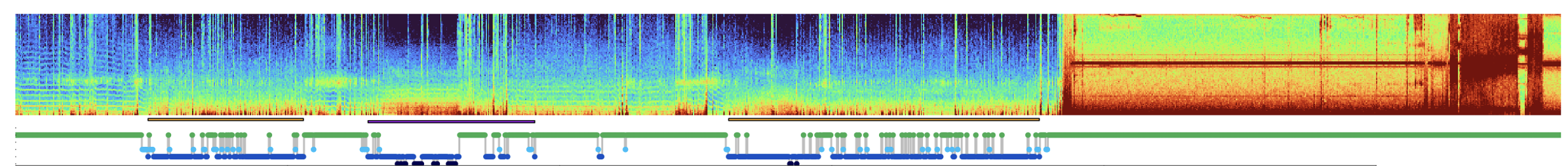
If not excluded manually during staging/EDF export, etc, it can be cumbersome for these periods to be included in downstream datasets:

they unnecessarily increase file size/processing time
often, these leading/trailing regions contain signals with excessively high (or low) amplitudes and/or variances, which can impact certain types of analysis, including automated sleep staging approaches if they normalize inputs across the whole recording (as Luna's POPS does): this can adversely impact the "true" or physiologic period of the recording, e.g. artificially restricting the range

The EDGER command attempts to define such regions - with a particular focus on finding contiguous intervals of leading and trailing artifact, distinct from noise occurring within the main portion of the recording. It also attempts to empirically define lights on/lights off times (or at least likely specific if not sensitive flagging of Lights On epochs). In principle, the behavior of EDGER would be very simple to do by eye via manual analysis: the goal here is to have something automated and reproducible.

Heuristic

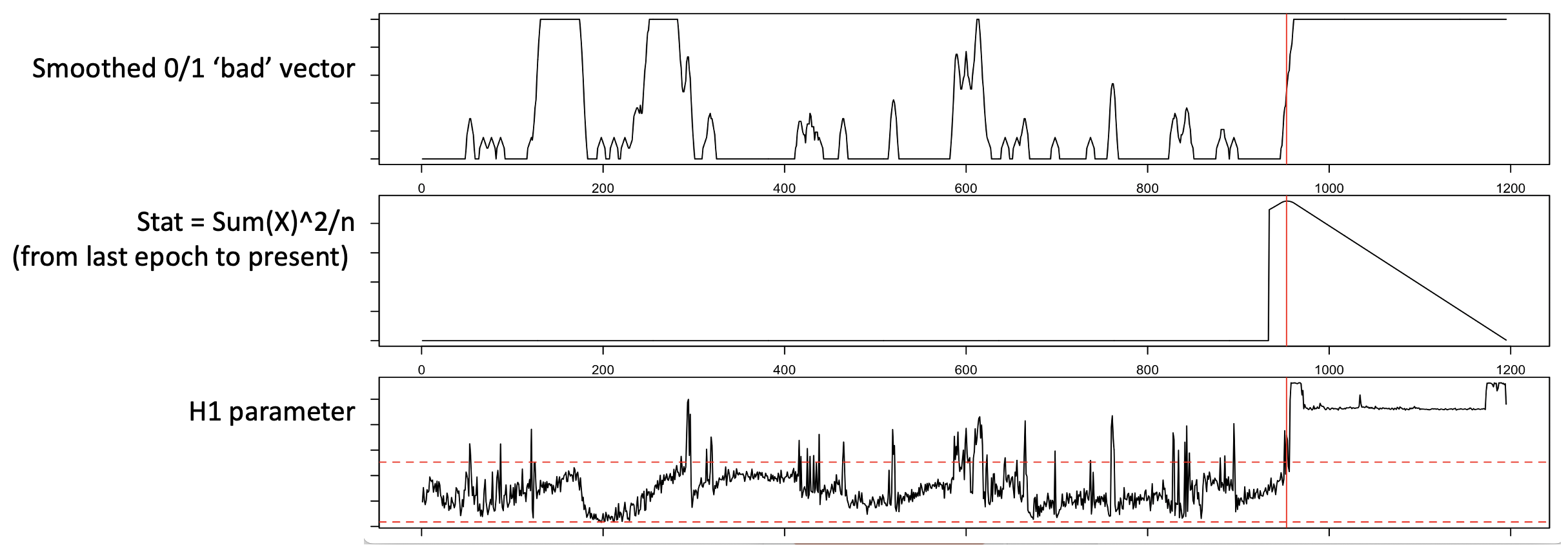
EDGER uses a very simple heuristic based on epochwise Hjorth parameters. For a single (EEG) channel, this plots the three parameters for a recording, showing a clear region at the end of the recording with excessively high amplitude (H1, on a log-scale) and low complexity (H3):

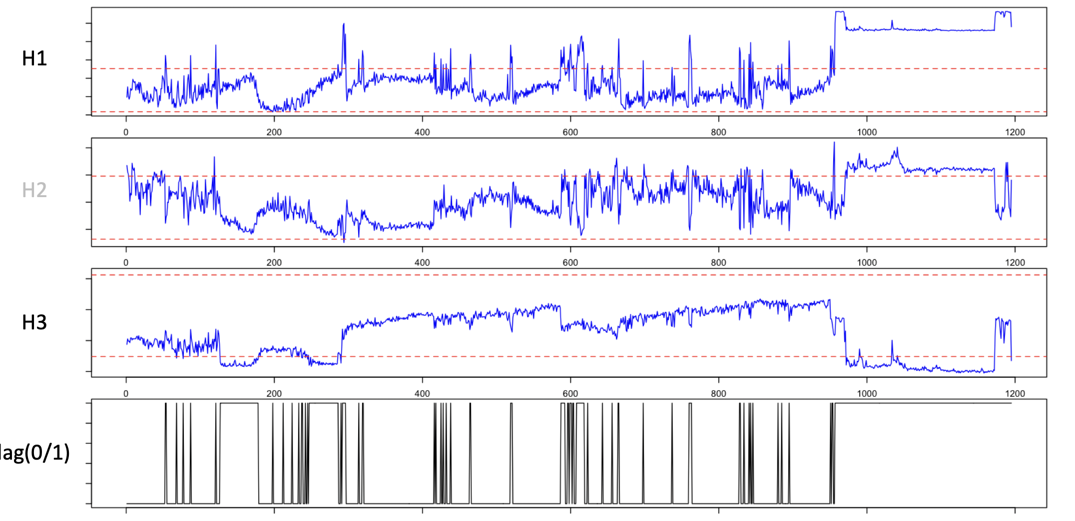
EDGER defines trailing/leading periods that are outliers as follows: if epochs are flagged as "good" or "bad" based on Hjorth-parameter thresholds, it defines a window that maximizes both the mean and total number of bad epochs at the edge:

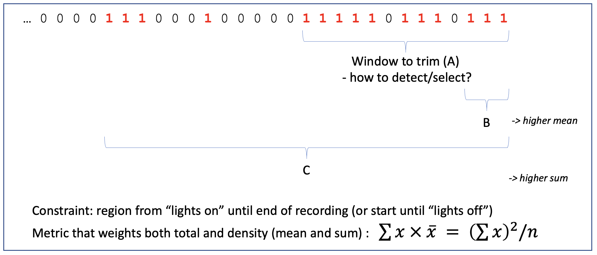
The above plot considers only the trailing window: a putative bad region is defined as that which maximizes the square of the count of bad epochs, divided by the number of epochs considered, moving out from the final epoch, to the last 2, then last 3, etc. Applied to real data, the middle panel shows this statistic and the maximum (red line):

In practice, EDGER performs the following steps:

smooths the epochwise 0/1 vector before selecting the cut-point, using a moving average with width +/-2mins (i.e. a 9 epoch window centered on each epoch).
it then flag epochs that are +/-3 SD units from median (th=2) for either H1 or H3, based on sleep epochs if the recording has sleep staging present; if no staging is present (or the option all is given) then it uses all epochs
it can consider only the leading or trailing periods with (only-start or only-end flags)
if it encouters more than 10 minutes (20 epochs, can be set with allow=20) of "clean" data (the statistic is 0), then do not flag any further after (or before) that point; that is, the goal is to set lights off/on, rather than avoid generically "bad data" per se.
if the maximum statistic implies fewer than 10 epochs (req=10) it will not set lights off/on annotations; i.e. if only a minor change would be made, not worth bothering, leave as is
if using multiple signals, it estimates the statistics separately for each, then picks the earliest lights-off and the latest lights-on
if cache=<name> is specified, this saves the estimates of lights-off and lights-on to the cache, in such a way that HYPNO, STAGE, POPS and SOAP will automatically use them to set epochs to L as appropriate.

Parameters

Parameter	Example	Description
`sig`	`C3,C4`	Restrict analysis to these channels
`cache`	`c1`	Saves the estimates of “lights-off” and “lights-on” such that HYPNO/STAGE/POPS/SOAP can use them to define.
`only-start`		Only consider leading artifact
`only-end`		Only consider trailing artifact
`allow`	`allow=20`	By default, do not allow more than 20 epochs of (10 mins) 'good' data at either end
`req`	`req=10`	By default, require equivalent of 10 epochs of bad data to be flagged
`w`	`w=9`	By default, smoothing window (total window, in epochs) - otherwise, 4 epochs either side (`w=9`)
`all`		Use all epochs to norm metrics (default: sleep only)
`wake`		Use only wake epochs to norm metrics (default: sleep only)
`h2`		Include second Hjorth parameter (default is not to)
`epoch`		Given output level information (same as `verbose`)

Output

Individual-level summaries (strata: none):

Variable	Description
`EOFF`	Eppch for lights off, if set (i.e. leading period trimming)
`LOFF`	Clock-time for lights off, if set (i.e. leading period trimming)
`EON`	Eppch for lights on, if set (i.e. leading period trimming)
`LON`	Clock-time for lights on, if set (i.e. leading period trimming)

Channel-level summaries (strata: CH):

Epoch-level summaries (options: epoch or verbose; strata: E x CH):

Variable	Description
`H1`	First Hjorth statisic
`H2`	Second Hjorth statisic (if `h2` set)
`H3`	Third Hjorth statisic
`FLAG`	Indicator of whether epoch is "bad" (0=good/1=bad)
`STAT`	Smoothed flag (0/1) indicator
`XON`	Primary statistic to determine lights on (trailing artifact)
`XOFF`	Primary statistic to determine lights off ( trailing artifact)
`TRIM`	Indicator (0/1) for whether this epoch should be trimmed

Examples

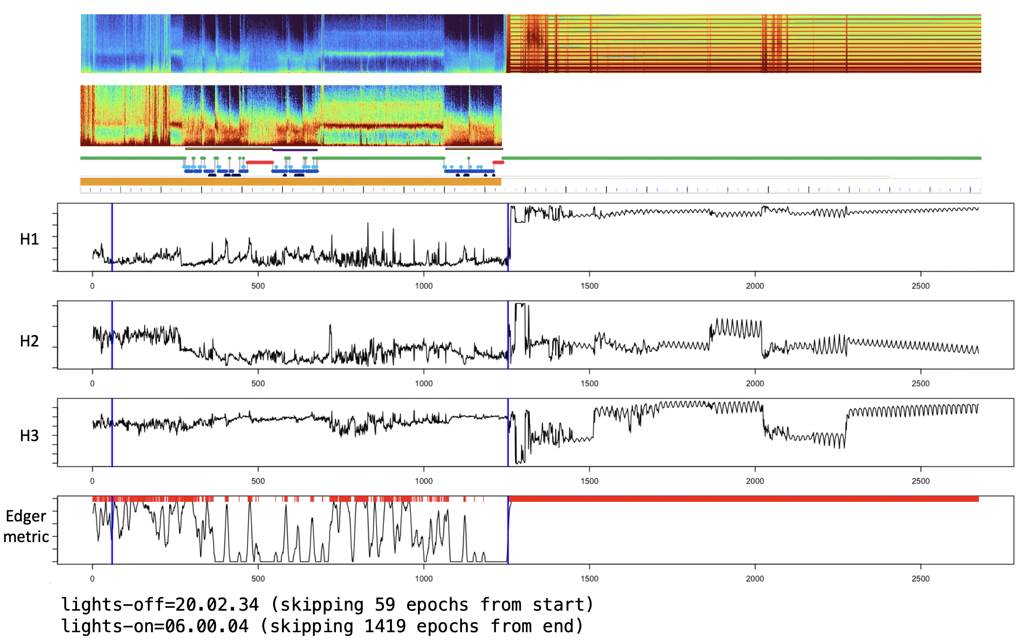
Based on the second individual from the tutorial dataset:

luna s.lst 2 -o out.db -s ' EDGER sig=EEG epoch cache=c1 & HYPNO cache=c1 '

 CMD #1: EDGER
   options: cache=c1 epoch sig=EEG
  set epochs to default 30 seconds, 1195 epochs
  skipping... cache c1 not found for this individual...
  set 0 leading/trailing sleep epochs to '?' (given end-wake=120 and end-sleep=5)
  anchoring on sleep epochs only for normative ranges, using 715 of 1195 epochs
  for EEG, flagged 279 epochs (H1=279, H3=0)
  H(1) bounds: 3.58692 .. 7.11721
  H(3) bounds: 0.411734 .. 2.39102
  setting cache c1 to store times
  lights-on=05.14.35 (skipping 241 epochs from end)

..................................................................
 CMD #2: HYPNO
   options: cache=c1 sig=*
  from TRIM cache, setting lights_on = 28590 secs, 476.5 mins from start
  set 242 final epochs to L based on a lights_on time of 28590 seconds from EDF start
  set 0 leading/trailing sleep epochs to '?' (given end-wake=120 and end-sleep=5)

In the above example, EDGER identifies over 200 epochs to skip, setting lights-on to 5:14:35am. As HYPNO is passed the cache option, it searches for lights-on (and also lights-off) values, and, if they exist, it will set epochs to L as appropriate.

Recordings with very extended periods of artifact

Note, in cases with very extended periods of artifact (e.g. at an extreme, could be longer than the sleep/clean period), this approach (based on statistical outliers) may fail to flag those regions with default setting, or if not anchored on pre-staged sleep epochs. For example, this recording has more than 12 hours of artifact:

With default settings, it correctly flags this period (as the default leverages sleep staging to normalize the metrics):

lights-on=06.00.04 (skipping 1419 epochs from end)

However, if applied to all epochs (adding all) as would be the case if staging were not avaialable, then

no trimming indicated: did not alter lights-off or lights-on times