Cross-signal analyses

Command	Description
`COH`	Pairwise channel coherence
`CORREL`	Pairwise channel correlation
`CC`	Coupling (dPAC) and connectivity (wPLI)
`PSI`	Phase slope index (PSI) connectivity metric
`XCORR`	Cross-correlation
`MI`	Mutual information
`TSYNC`	Cross-correlation and phase delay (alternate implementation)
`GP`	Granger prediction

COH

Calculates pairwise spectral coherence across channels

The COH function calculates the magnitude-squared coherence for pairs of signals with similar sampling rates.

Parameters

Parameter	Example	Description
`sig`	`sig=C3,C4`	An optional parameter, to specify which channels to calculate pairwise coherence between
`sig1`	`sig1=C3,C3`	In stead of `sig`, specify all `sig1` by `sig2` channel pairs
`sig2`	`sig2=F3,F4`	As above
`sr`	`sr=125`	Optionally, set sample rates to `sr` if different for a particular channel (i.e. to ensure that all signals have similar sampling rates
`spectrum`	`spectrum`	Output full cross-spectra coherence rather than just in frequency bands (delta, theta, etc)
`epoch`	`epoch`	A flag to output coherence statistics for per epoch as well as the whole signal
`epoch-spectrum`	`epoch-spectrum`	A flag to output full cross-spectra coherence statistics for each epoch/channel pair

Warning

If requesting the full spectrum and epoch-level analyses for a large number of channels, the output database may be very large... In this case, you should use text-table mode output (with -t) for better performance when working with the output (as destrat can be slow othewise, for datasets with very large numbers of strata).

Using sig1 and sig2 instead of sig can be more efficient, if you are only interested in particular combinations of pairs. For example, to see the pairwsie coherences between one channel and four others:

 sig1=C3 sig2=F3,F4,O1,O2

This will only evaluate four pairs (whereas sig=C3,F3,F4,O1,O2 would evaluate 10 pairs, even if some pairwise comparisons are not of interest).

Output

Coherence for power bands (B x CH1 x CH2)

Variable	Description
`COH`	Magnitude-squared coherence
`ICOH`	Imaginary coherence
`LCOH`	Lagged coherence

Full cross-spectra coherence (option: spectrum, strata: F x CH1 x CH2)

Variable	Description
`COH`	Magnitude-squared coherence
`ICOH`	Imaginary coherence
`LCOH`	Lagged coherence

Coherence for power bands, per epoch (option: epoch, strata: E x B x CH1 x CH2)

Variable	Description
`COH`	Magnitude-squared coherence
`ICOH`	Imaginary coherence
`LCOH`	Lagged coherence

Full cross-spectra, per epoch (option: epoch and spectrum, strata: E x F x CH1 x CH2)

Variable	Description
`COH`	Magnitude-squared coherence
`ICOH`	Imaginary coherence
`LCOH`	Lagged coherence

nb. references for methods to be added

Example

To estimate the cross-spectra (up to 20 Hz) between the two EEG channels during NREM2 sleep for the tutorial individual nsrr02:

luna s.lst nsrr02 -o out.db -s "MASK ifnot=NREM2 & RE \
                                & COH spectrum max=20 sig=EEG,EEG(sec)"

Loading this into lunaR,

k <- ldb( "out.db" )

and extracting the relevant data frame:

d <- lx(k,"COH","CH1","CH2","F")

and plotting:

plot( d$F, d$COH , type="l" , 
      xlab="Frequency (Hz)" , ylab="Coherence" , 
      ylim=c(0,1) , lwd=2, col="red")

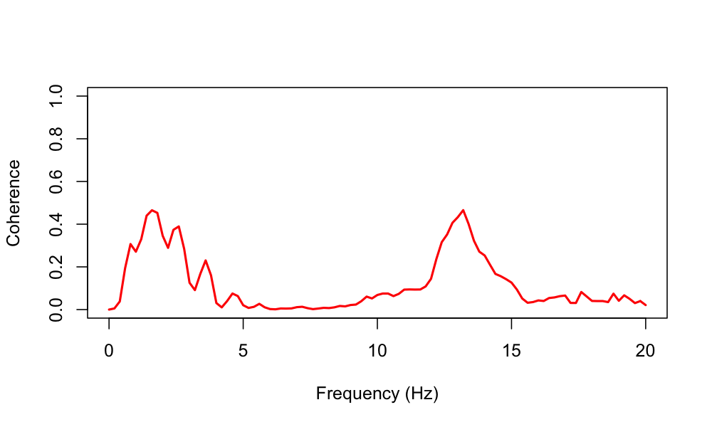
Following other reports (for example), we see peaks in EEG coherence especially for the low delta and sigma frequencies during NREM sleep. Naturally, the precise interpretation of coherence analysis (like any sleep EEG analysis) depends on the exact choice of montages, referencing and other technical and subject-level details, not to mention the potential for artifact (e.g. as illustrated here).

CORREL

Calculates pairwise Pearson correlation between signals

CORREL estimates pairwise correlation coefficients between signals, either for the whole signal, or epoch-by-epoch. When epoch-level statistics are requested, Luna also reports the mean and median of all per-epoch statistics for a given channel pair.

As of v0.27, Luna also provides functions to incorporate spatial channel distance (i.e. for the EEG/MEG context) of channels, and to find disjoint sets of highly correlated channels.

Parameters

Parameter	Example	Description
`sig`	`sig=C3,C4,F3,F4`	Optionally specify which signals to correlate (otherwise, do all)
`sig1`	`sig=C3,C4`	Alternatively, only evaluate all `sig1` by `sig2` pairs
`sig2`	`sig=F3,F4`	As above
`sr`	`sr=128`	Resample channels to this sample rate, if they are not already at that rate
`epoch`	`epoch`	Display per-epoch correlations, and estimate mean and median correlation across epochs

Epoch-level correlations

By default, the correlations from CORREL are based on the entire signal. To instead estimate of channel-pair correlations based on aggregating epoch-level correlations, use the ch-epoch option. This is often likely more robust to artifacts. In particular, if you also use ch-median then the final correlation is the median of epoch-level correlations (otherwise, default = mean). In general, when using the CORREL command, it is probably advisable to always add ch-epoch ch-median.

Parameter	Example	Description
`ch-epoch`		Base overall correlations on aggregate summaries of epoch-level correlations
`ch-median`		Use the median (instead of the mean) when applying `ch-epoch`

Including EEG channel topographies

For high-density EEG/MEG studies, CORREL can produce some simple metrics that flag pairs of channels that are more correlated by might be expected given their topographical similarity. This may be indicative of artifact or bridging, etc.

To include spatial distances in correlations, it is first necessary to have previously attached a set of channel locations via the CLOCS command) prior to running CORREL. An example map (for a 64-channel EEG) can be found here: e.g.

  CLOCS clocs=clocs64
  CORREL sig=${eeg}

Channel locations are translated to a cosine similarity (-1 to +1, where +1 is most similar) and are output as the S variables from the CORREL command:

   destrat out.db +CORREL -r CH1 CH2

This allows easy plotting of correlation against spatial proximity, e.g. to spot extreme outliers. (Note: assuming the same map has been used, S will obviously be the same of all individuals.)

ch-spatial-threshold ch-spatial-weight to CORREL,

Disjoint sets of highly correlated channels

CORREL now prints disjoint sets of highly-correlated channels (as defined by the ch-high option) channels, with CHS stratifier, if the ch-high option is given.

Output

Whole-signal correlations for pairs of channels (strata: CH1 x CH2)

Variable	Description
`R`	Pearson product moment correlation
`R_MEAN`	(If `epoch` is specified) the mean of epoch-level correlations
`R_MEDIAN`	(If `epoch` is specified) the median of epoch-level correlations
`S`	If channel locations attached for this pair, the cosine similarity (based only on map)

Whole-signal correlations for pairs of channels (option: epoch, strata: E x CH1 x CH2)

Variable	Description
`R`	Per-epoch Pearson product moment correlation

Channel-level summaries (strata: CH)

Variable	Description
`SUMM_MEAN`	Mean correlation with all other channels
`SUMM_N`	Number of other channels this is correlated with
`SUMM_MIN`	Minimim correlation for this channel
`SUMM_MAX`	Maximum correlation for this channel
`SUMM_HIGH`	Number of correlations (i.e. channels) above `ch-high`
`SUMM_LOW`	Number of correlations (i.e. channels) below `ch-low`

Disjoint sets of highly correlated channels (potion: ch-high, strata: none )

Variable	Description
`SUMM_HIGH_N`	Total number of disjoint sets in the data
`SUMM_HIGH_CHS`	Comma-delimited list of channnels in this highly-correlated set

Disjoint sets of highly correlated channels (option: ch-high, strata: CHS)

Variable	Description
`N`	Number of channels in this disjoint set
`SET`	Channels in this disjoint set

Example

Here we consider the epoch-by-epoch correlation between the two EOG channels for tutorial subject nsrr02. Using lunaC to estimate and report correlations at the epoch level:

luna s.lst nsrr02 -o out.db -s "MASK if=wake & RE \
                                & STAGE \
                                & CORREL epoch verbose sig=EOG(L),EOG(R)"

Note that the above command also reports the manually-assigned stage of each epoch (with the STAGE command, which we can use later when plotting results:

Using lunaR to examine the output (in R):

library(luna)

We'll attach the output database just created:

k <- ldb( "out.db" )

Examining the contents with lx():

lx(k)

CORREL : CH1_CH2 CH1_CH2_E 
MASK : EPOCH_MASK 
RE : BL 
STAGE : E

First, we'll extract a simple vector of sleep stage (the STAGE variable from the STAGE command):

ss <- lx( k , "STAGE" , "E" )$STAGE

Second, we'll extract the epoch-by-epoch correlations:

d <- lx( k , "CORREL" , "CH1" , "CH2" , "E" )

Viewing data-frame d, note that the epochs (E) do not start at 1, because we previously restricted this analysis to sleep epochs:

head(d)

      ID    CH1    CH2   E         R
1 nsrr02 EOG(L) EOG(R)  92 0.5052592
2 nsrr02 EOG(L) EOG(R)  93 0.7998685
3 nsrr02 EOG(L) EOG(R)  98 0.4698097
4 nsrr02 EOG(L) EOG(R)  99 0.3147986
5 nsrr02 EOG(L) EOG(R) 100 0.3153311
6 nsrr02 EOG(L) EOG(R) 101 0.6581321

Finally, we can plot these epochs:

plot( d$E , d$R , col = lstgcols( ss ) , pch=20 , ylab="L-R EOG correlation", xlab="Epoch", ylim=c(-1,1) )
abline( h=0 , lty=2 )

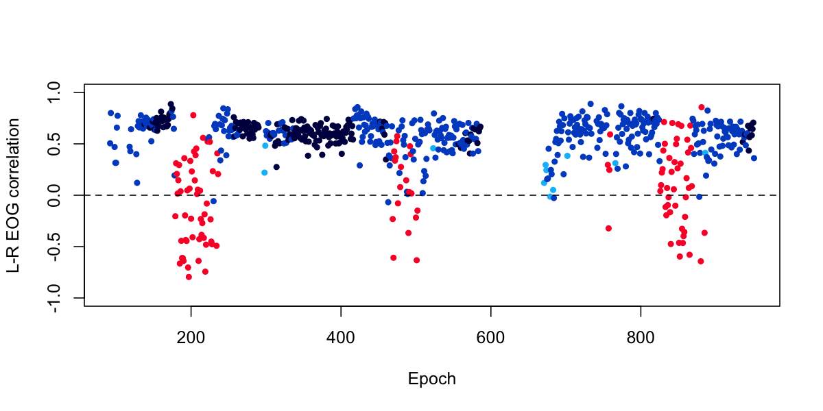
For this particular individual, there seems to be a clear and interesting pattern, in which we see that REM epochs (in red) are more likely to show negative correlations between the left and right EOG, reflecting the deviations due to eye-movements during REM.

Disjoint sets of highly correlated channels

CORREL now prints disjoint sets of highly-correlated channels (as defined by the ch-high option): channels, with CHS stratifier, e.g.

destrat out.db +CORREL -r CHS

ID     CHS     N       SET
ID01   1       2       Fp2,AF4
ID01   2       2       F3,F1
ID01   3       3       F2,FC2,FZ
ID01   4       6       C2,CP2,P2,P4,CPZ,PZ
ID01   5       2       CP4,CP6
ID01   6       2       P3,P1
ID01   7       2       P6,P8
ID01   8       4       PO4,O2,POz,OZ

i.e. here we have 8 groups (CHS), where N is the number of channels in that group.

The baseline CORREL output will list the total # of channels with a highly-correlated partners:

destrat out.db +CORREL

ID    SUMM_HIGH_CHS                     SUMM_HIGH_N
ID01  CPZ,P4                            2
ID02  NA                                0
ID03  NA                                0
ID04  CP2,CP6                           2
ID05  NA                                0
ID06  NA                                0
ID07  P3,TP7                            2
ID08  P1,P2,P7,P8                       4
ID09  CP2,O2,OZ,P4,POz                  5
ID10  NA                                0
ID11  AF4,C4,CP2,CP6,F2,F4,F6,FC2,FC4   9
ID11  P1,P7                             2
ID12  AF4,FC4,P4,TP8                    4
... etc ...

Spatial thresholding

Note that these statistics/sets are optionally influenced by ch-spatial-threshold, which only includes channel pairs that are below a certain similarity (i.e. not neighbouring). You can look at the distribution of S from the output of +COREEL -r CH1 CH2 (see above). Based on the above example map with 57 channels present in the EDF, something like 0.8 excludes ~222 out of the ~1600 pairs, i.e. on average, this will exclude the closest ~4 channels for each channel (4 * 57 = 228). Valid arguments are between -1 and +1.

With spatial thresholding, channel pairs with a spatial similarity above threshold are excluded from all correlational analyses. The column SUMM_N gives the number of included channels after these step.

  CORREL  sig=${eeg} ch-epoch ch-spatial-threshold=0.8 ch-high=0.98 '

i.e.

luna s.lst -o out.db \
           -s 'CLOCS file=clocs64
           REFERENCE sig=${eeg} ref=A1,A2
           CORREL sig=${eeg} ch-epoch ch-spatial-threshold=0.8 ch-high=0.98 '

Spatial weighting

The argument ch-spatial-weight only impacts the SUMM_MEAN output, which is the mean of the absolute value of correlations for a channel, with all other channels. (Note, this used not to take the absolute value, but I've changed this behavior just now, along w/ the other changes to CORREL).

As above, SUMM_MEAN may be based on epoch-level stats (after taking the mean/median of those) or on whole-recording signals. In addition, SUMM_MEAN is only based on below threshold channel pairs, if ch-spatial-threshold has been set. Setting ch-spatial-weight will weight the correlation, multiplying each absolute correlation by a weight factor determine by the cosine similarity between the channel pairs, before summing for that channel. The weight is set such that more nearby channels have less weight -- i.e. if one is trying to pick up on more distal channel pairs that still have high correlations in the signals.

Luna defines the weight as:

  W = ( ( 1 - S ) / 2 )^X

i.e. we scale similarity S from ( -1 , +1 ) to ( 0 , 1 ) and then we optionally take the X^th power, i.e. so that higher X values more we put even less weight on nearby channel pairs. The default is 2. e.g. for a linear effect, use:

ch-spatial-weight=1

CC

Calculates coupling and connectivity metrics

The CC command estimates cross-frequency coupling (currently dPAC) and, for inter-channel connectivity, the weighted phase lag index (wPLI). It implements a time-shifting randomization to generate the null distributions of these metrics.

Note

Although CC currently only implements these two metrics, in future releases other coupling and connectivity metrics will be added within this framework (e.g. the coherence metrics currently performed using COH).

For one of more signals, phase-amplitude coupling is estimated by the dPAC method, if the pac option is specified. The phase and amplitude of the signal is estimated using wavelets, with center frequencies of fc and fc2 for phase and amplitude components respectively, where fc is expected to be of lower frequency than fc2. Multiple frequencies for either the phase (fc) or amplitude (fc2) can be specified with a comma-delimited list, e.g. fc=1,2,4. Alternatively, a grid of frequencies cab be specified by using fc-range=1,20 instead of fc; here, it is also required to specify num, e.g. num=20, which generates 20 fc values evenly spaced on a log scale, between 1Hz and 20Hz. The linear option will force the grid to be uniform on a linear, not log, scale instead. When considering phase-amplitude coupling, only pairs where the phase frequency (fc) is lower than the amplitude frequency (fc2) are retained for analysis.

As well as the wavelet center frequency, one can specify the bandwidth of the wavelet, via the wavelet time-domain full width at half maximum (FWHM), following this convention. See the CWT-DESIGN command for more details, i.e. to better understand the implication of setting a particular FWHM for the frequency domain properties of the wavelet. In general, smaller FWHM values (in the time-domain) correspond to broader FWHM in the frequency domain (i.e. a wider range of frequencies above and below the center frequency will be captured).

Default FWHM values

If no FWHM values are specified, Luna will use a default value based on the frequency of the wavelet. For this, we seed on the default values selected in the Cox & Fell manuscript described in this vignette. In that manuscript, they used wavelet center frequencies of 0.5 to 30 Hz, evenly spaced on a log space, and paired these with 35 FWHM values evenly-spaced on a log scale from 5 to 0.25. For an arbitrary frequency, Luna will therefore use the following relation to generate a reasonable default value for the FWHM, which maintains equal frequency domain FWHM values on a log-scale:

exp(-0.7316762 * ln(F) + 1.1022791 )

Parameters

Core parameters

Parameter	Example	Description
`sig`	`sig=C3,C4`	Optionally specify channels (default is to include all)
`fc`	`fc=11,15`	Specify wavelet center frequency/frequencies (phase)
`fwhm`	`fwhm=1,1`	Wavelet FWHM value(s) (phase)
`fc2`	`fc2=11,15`	For PAC: as `fc` for amplitude
`fwhm2`	`fwhm2=1,1`	For PAC: as `fwhm` for amplitude
`nreps`	`nreps=1000`	Number of randomized, surrogate time series generated
`pac`	`pac`	Estimate within-channel phase-amplitude coupling metrics
`xch`	`xch`	Estimate between-channel connectivity metrics

Secondary parameters (primarily for specifying grids of frequency/FWHMs to test)

Parameter	Example	Description
`fc-range`	`fc-range=1,20`	Specify range of center frequencies (requires `num`) (phase)
`fwhm-range`	`fwhm-range=5,0.25`	Specify range of FWHM values (requires `num`) (phase)
`num`	`num=20`	Number of intervals (evenly spaced on log scale) for `fc-range` or `fwhm-range` (phase)
`fc-range2`	`fc-range2=1,20`	For PAC: as `fc-range2` for amplitude
`fwhm-range2`	`fwhm-range2=5,0.25`	For PAC: as `fwhm-range2` for amplitude
`num2`	`num2=20`	For PAC: as `num` for amplitude
`length`	`length=10`	Wavelet duration (in seconds)
`linear`	`linear`	For ranges (e.g. `fc-range`) evenly space on a linear scale
`no-epoch-output`	`no-epoch-output`	Suppress all epoch-level output

That is, fc-range and num would be used instead of fc, etc.

Output

Whole-signal level metrics (strata: CH1 x CH2 x F1 x F2)

Variable	Description
`CFC`	0/1 for whether this metric is a cross-frequency contrast (i.e. `F1` != `F2`)
`XCH`	0/1 for whether this metric is a cross-channel contrast (i.e. `CH1` != `CH2` )
`dPAC`	Debiased phase-amplitude coupling metric
`dPAC_Z`	Empirical Z-score for `dPAC` based on time-shuffling
`wPLI`	Weighted phase-lag index connectivity metric
`wPLI_Z`	Empirical Z-score for `wPLI` based on time-shuffling

Epoch-level metrics (strata: E x CH1 x CH2 x F1 x F2)

Variable	Description
`dPAC`	Debiased phase-amplitude coupling metric
`dPAC_Z`	Empirical Z-score for `dPAC` based on time-shuffling
`wPLI`	Weighted phase-lag index connectivity metric
`wPLI_Z`	Empirical Z-score for `wPLI` based on time-shuffling

Example

See this vignette for an application of both dPAC and wPLI metrics.

Here, using two EEG channels from the second individual in the tutorial dataset, we extract only N2 sleep at consider wPLI between the two channels at a grid of 50 frequencies, linearly spaced between 1 and 25 Hz:

luna s.lst 2 -o out.db
             -s 'MASK ifnot=NREM2 & RE &
                 CC sig=EEG,EEG(sec) fc-range=1,25 num=50 nreps=200 linear xch'

Extracting the output as follows:

destrat out.db +CC -r F1 F2 CH1 CH2

We can plot the wPLI (left) and correspondong Z-score (the empirical value derived from randomization, right):

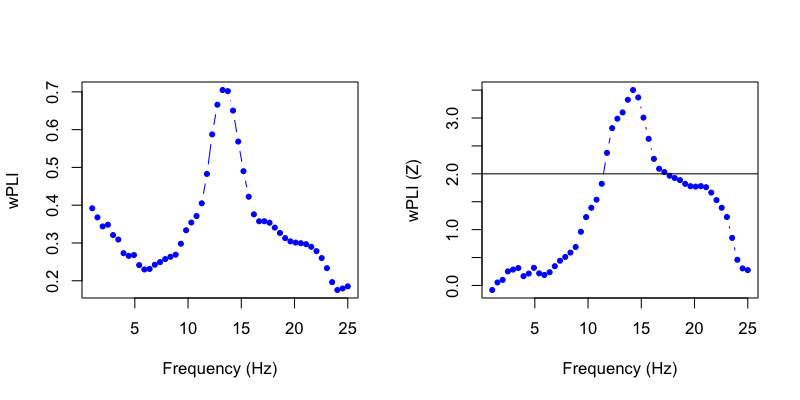
That is, we see significant connectivity between these two central channels in the spindle/sigma frequency band during N2 sleep.

Scaling the number of tests

Although this is designed to run reasonably efficiently, if you have lots of channels and/or lots of frequencies and want to look at cross-frequency coupling between all pairs, then run time can get slow (...very slow...) especially if you are using randomization to estimate Z scores (nreps) and/or have lots of individuals in the datasets. Therefore, try to focus these analyses and start small...

PSI

Calculates the phase slope index across channels

Estimates the phase slop index between pairs of channels, and provides a single-channel summary of net PSI (i.e. net sender versus recipient).

The command requires that channels have similar sampling rates.

Parameters

To set the frequency or frequencies at which to calculate PSI either:

specify f and w - one or more frequencies, for bands f-w/2 to f+w/2
or specify f-lwr, f-upr only - for a band of lower to upper (or an equal range of comma-delimited values for each to give a range of bands, e.g. f-lwr=1,4,8 and f-upr=4,8,12 implies three bands: 1-4 Hz, 4-8 Hz and 8-12 Hz)
or specify f-lwr, f-upr, w and r - for a range of bands, from f equalling f-lwr up to f-upr, in steps of r Hz; for each frequency, the window of w spanning the center frequency is constructed

Parameter	Example	Description
`sig`	`sig=C3,C4`	An optional parameter, to specify which channels to calculate PSI
`epoch`		Report epoch-level (e.g. 30-second epoch) output
`f-lwr`	`f-lwr=3`	Consider frequencies from `f-lwr` to `f-upr` (as a band, or in steps of `r` )
`f`	`f=10,12,15`	One or more frequencies to test (Hz)
`w`	`w=5`	Window around each center frequency (Hz) in which to calculate PSI

Secondary parameters are:

Parameter	Example	Description
`eplen`	`eplen=5`	PSI sub-epoch length (default 4 seconds)
`seglen`	`seglen=2.5`	Segment length (with 50% overlap) within each sub-epoch
`cache-metrics`	`cache-metrics=c1`	Cache PSI, e.g. for use with `PSC`

Cache options

Parameter	Example	Description
`cache-metrics`	`cache-metrics=c1`	Cache net and pairwsie `PSC` (e.g. for `PSC`)

Output

Analysis parameter output (strata: F )

Variable	Description
`F1`	Lower frequency
`F2`	Higher frequency
`NF`	Number of frequency bins

Channel-level output (strata: CH )

Variable	Description
`PSI`	Net PSI (standardized) for this channel

Channel pair output (strata: CH1 x CH2)

Variable	Description
`PSI`	Standardized PSI for this channel pair
`PSI_RAW`	Raw PSI
`STD`	Standard deviation of PSI

Channel-level output (option: epoch, strata: E x CH )

Variable	Description
`PSI`	Net PSI (standardized) for this channel

Channel pair output (olption: epoch, strata: E x CH1 x CH2)

Variable	Description
`PSI`	Standardized PSI for this channel pair
`PSI_RAW`	Raw PSI
`STD`	Standard deviation of PSI

Example

to be added

XCORR

Efficient cross-correlation analysis

This command computes pairwise cross-correlations between signals using the FFT. All channels must have similar sample rates. This can be performed either epoch-wise, or on the whole signal. It computes correlations for a window of a fixed number of seconds w, optionally with an offset c (i.e. to find the maximum correlation of alignments from c-w to c+w seconds.

Parameters

Parameter	Description
`sig`	Restrict analysis to these channels (at least two required)
`epoch`	Epoch-wise analysis
`w`	Optionally, maximum shift/window size to consider (seconds)
`c`	Optionally, offset to add (see above) (seconds)
`verbose`	Give verbose output

Output

Pairwise channel measures for whole recording (option: epoch; strata: CH1 x CH2):

Variable	Description
`D_MN`	Mean delay over epochs (seconds)
`D_MD`	Median delay over epochs (seconds)
`S_MN`	Mean delay over epochs (samples)
`S_MD`	Median delay over epochs (samples)
`D`	Delay based on average of lagged XCs (seconds)
`S`	Delay based on average of lagged XCs (samples)

Pairwise cross-correlations for a given sample delay D (option: verbose; strata: D x CH1 x CH2):

Variable	Description
`T`	Lag in seconds
`XC`	Cross-correlation

Examples

MI

Calculates pairwise mutual information metrics across channels

Estimates mutual information, a measure of dependence between two signals, based on methods described in Analyzing Neural Time Series Data by MX Cohen. Total correlation and dual total correlation are two normalized variants of the mutual information statistic: MI / min[ H(X), H(Y) ] and MI/H(X,Y) respectively, where MI is mutual information, H(X) and H(Y) are the marginal entropies, and H(X,Y) is the joint entropy.

Signals are first coarse-grained: the number of bins is determined by one of three rules: Freedman-Diaconis (default), Scott or Sturges rule, as described in Cohen.

Parameters

Parameter	Example	Description
`sig`	`sig=C3,C4,F3,F4`	Optionally specify channels (default is to include all)
`epoch`	`epoch`	Calculate and report MI and other measures per epoch
`scott`	`scott`	Use Scott's rule to determine bin number
`sturges`	`sturges`	Use Sturges' rule to determine bin number
`permute`	`permute=1000`	Estimate empirical significance via permutation, e.g. with 1000 null replicates

Alert

Permutation and epoch-level analyses with the MI command can be relatively slow .

Output

Output for the whole signal (strata: CH1 x CH2)

Variable	Description
`MI`	Mutual information
`TOTCORR`	Total correlation
`DTOTCORR`	Dual total correlation
`JINF`	Joint entropy
`INFA`	Marginal entropy of first signal
`INFB`	Marginal entropy of second signal
`NBINS`	Number of bins

Output per-epoch, with epoch (option: epoch, strata: CH1 x CH2)

Variable	Description
`MI`	Mutual information
`TOTCORR`	Total correlation
`DTOTCORR`	Dual total correlation
`JINF`	Joint entropy
`INFA`	Marginal entropy of first signal
`INFB`	Marginal entropy of second signal

Output for permutation test (option: permute)

Variable	Description
`EMP`	Empirical p-value for mutual information statistic
`Z`	Z-statistic

TSYNC

Cross-correlation and phase delay

This function is now redundant - use XCORR instead

Estimate the cross-correlation between two signals, within a window of W seconds, and report the estimated phase delay (in seconds) based on the maximal cross-correlation in that time window.

Options

Parameter	Example	Description
`sig`	`sig=C3,C4,F3,F4`	Optionally specify channels (default is to include all)
`w`	`w=0.5`	Required time window (seconds)
`verbose`		Verbose output
`epoch`		Epoch-level output

Output

Channel-pair output (strata: CH1 x CH2)

Variable	Description
`S`	Phase delay based on cross-correlation

Channel-pair output (option: verbose, strata: D x CH1 x CH2)

Variable	Description
`XCORR`	Estimated cross-correlation for this delay

Epoch-level channel-pair output (option: epoch, strata: CH1 x CH2)

Variable	Description
`S`	Phase delay based on cross-correlation

Example

to be added

GP

Applies Granger prediction

Parameters

Parameter	Example	Description
`sig`	`sig=C3,C4,F3,F4`	Optionally specify channels (default is to include all)

Output

Channel-pair output (strata: CH1 x CH2)

Variable	Description

Example

to be added